
LETTER
Development of Contactless Sand Production Test Instrument
Huiqin Jia*, Ruirong Dang
Article Information

Identifiers and Pagination:
Year: 2017Volume: 10
First Page: 1
Last Page: 11
Publisher Id: TOPEJ-10-1
DOI: 10.2174/1874834101701010001
Article History:
Received Date: 08/09/2016Revision Received Date: 28/10/2016
Acceptance Date: 02/11/2016
Electronic publication date: 12/01/2017
Collection year: 2017
open-access license: This is an open access article licensed under the terms of the Creative Commons Attribution-Non-Commercial 4.0 International Public License (CC BY-NC 4.0) (https://creativecommons.org/licenses/by-nc/4.0/legalcode), which permits unrestricted, non-commercial use, distribution and reproduction in any medium, provided the work is properly cited.
Abstract
Background:
Sand production is an important factor affecting reservoir exploitation. Excessive sand production affects the oil well life, causes the damage to the oil recovery device and brings serious hidden danger in the process of safety production.
Objective:
This paper presents a sand content computation model for the crude oil, which uses the power of sand production and Parseval theorem, develops a system to monitor the sand content.
Method:
The main problem of designing the mechanical structure and matching layer for sand sensor is introduced. Furthermore a contactless Doppler ultrasonic method is used to develop sand amount detection system‚ finally the system measurement accuracy is calibrated by the developed calibration system.
Conclusion:
The sand production computation model can describe the relationship between sand monitor output and sand amount; compute the oil sand carrying ratio. The sand sensor is installed on the outside of pipe, not directly contacted with the sand particles. Measurement accuracy of the sand production is higher than the same type instrument.
1. INTRODUCTION
Sand production is often encountered in the oil development process. Because it not only causes a lot of troubles to the production process, but also impacts reservoir oil recovery rate and oil & gas recovery, leads to serious hole collapse, causes damage and well abandonment [1]. Only the appropriate sand production can guarantee the normal production, which requires monitoring sand production situation, timely detects abnormal phenomenon, takes sand plugging measures. Some petroleum instrument development companies have developed the multiphase fluid sand monitoring system. For example, the Danish Clampon company developed sand monitoring system DSP-06, which is developed based on the “Clamp smart ultrasonic sensor” technology [2], but the measurement accuracy cannot meet the field measurement requirements. The main reasons are as follows: There didn’t have a mature sand production monitoring model, the most system uses the sand production model described previously, which gives a sand production calculation model [3]. The shortcoming of this model is less consideration of flow velocity, background noise and sand diameter. So the measurement result varies with the test condition, moreover the sand production cannot be calibrated by it. Other systems use the acceleration sensor to detect the sand of high frequency vibration on the pipelines; the shortcoming of that system is the high measurement errors for low velocity and must stop oil transportation to install it. This paper presents a contactless sand detection method, designs the acoustic signal detection sensor and acoustic sand signal detection circuit, finally gives the calibration method and measurement result [4, 5].
2. MODEL DERIVATION FOR SAND PRODUCTION
When a sand particle strikes the pipe wall, then a weak ultrasonic pulse created, which is a dynamic random signal. If there are n sand particles striking the pipe wall within the ΔT time at the velocity of V, the average power S through pipe transmission can be given as equation (1) [6]:
 |
(1) |
Where: S = the signal average power in the ΔT time
K1 = a constant
mi = the sand particle mass, i from 1 to n
Δt = sampling interval.
The sand mass in the period of ΔT is presented as equation (2):
 |
(2) |
Substituting equation (2) into equation (1), then can obtain equation (3):
 |
(3) |
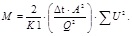
M can be obtained from equation (3):
 |
(4) |
Where: M = the sand particle mass in the ΔT time.
It was also assumed that the average velocity of n sand particles is equal to the flow velocity V, and
 , substituting V into equation (4), obtains equation (5):
 |
(5) |
Where: Q =instantaneous volume flow
A = Pipe cross-sectional area
Additionally, According to the Parseval theorem [7], we can obtain the average power S of digitized sand signal within the ΔT time:
 |
(6) |
Substituting equation (6) into equation (5), can obtain the equation (7):
 |
(7) |
 |
(8) |
Substituting equation (8) into equation (7), then the accumulated sand production M is obtained:
 |
(9) |
 |
(10) |
Where Un = The Output of background noise signal.
Us = The output signal including background noise.
Then we can calculate the sand ratio R from equation (9):
 |
(11) |
Where Q1= total mixture volume flow through the pipeline in the ΔT time.
Seen from equation (9), Pipe cross sectional area A is a constant. Moreover the sampling rate is a constant, so the sampling interval Δt is fixed. If the instantaneous flow Q and the voltage of sand production signal U are known, then the calibration constant K can be obtained through experiment, which relates to flow velocity and the size of sand particles. Therefore the total sand quality M can be computed by the equation (7). The sand ratio R can be computed by equation (11) if the total volume flow Q1 is known.
3. SYSTEM DESIGN
3.1. Experimental Setup
The diagram of sand signal detection system is shown in Fig. (1), which contains Instantaneous Sand Production Sub-System (ISPSS) and Sand Production Signal Amplitude Obtaining Sub-System(SPSAOSS), ISPSS can obtain the flow Q1 and Q. SPSAOSS can obtain the amplitude U of sand signal.
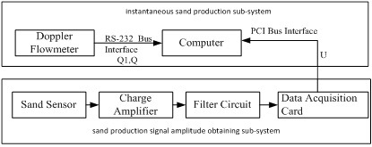 |
Fig. (1). Principle block diagram for sand production signal detection system. |
Doppler Flow meter shown in Fig. (1) is designed based on the Doppler technology, which can obtain Q. This method is described in the literature [8]. Because the sampling number can be counted through computer, then Q1 is fixed. So the R can be easily computed through equation (11), then the value of R transfers to the computer through the RS-232 bus. The high resister charge signal shown in the Fig. (2) is amplified to the low resister voltage one, which function is to realize impedance transformation. In addition, frequency distribution of sand signal has curtain range, sometimes it exceeds the scope due to the noise generated by pipe vibration, so the first thing is to filter the noise signal, then acquires the amplitude U of sand signal through the PCI bus of data acquisition card.
3.2. Design of Sand Sensor
The structure of sand sensor is shown in Fig. (2), which contains sensitive elements, matching layer, shell and installation mount. The shell of which is made of aluminum, a concave groove is convenient to the install on the pipe outer wall using the fixed belt clip, the materials of which is piezoelectric ceramics. The piezoelectric ceramic piece uses the PSnN-51, and Piezoelectric wafer is thin wafer type, which vibrates along the thickness direction. The produced ultrasonic wave is a longitudinal one [9].
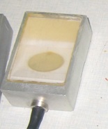 |
Fig. (2). Structure of sand production sensor. |
Sand production sensor only needs to fix on the oil pipe, so it’s contactless to the mixture inside of the pipe. Therefore it does not affect the normal work of the oil and gas transportation process system.
3.3. Optimization of Sand Sensor Installation Location
We build the bend pipe model using Fluent software to determine the best location of sand sensor. The material of pipe is stainless steel. The parameters of pipe model are as follows: thickness of pipe wall is 0.004m; the Pipe diameter is 0.08m; the straight pipes of bend pipe is 20m; circular arc radius is 4m; Young’s modulus of stainless steel is 206GPa; poisson ratio is 0.29; the young's modulus of water is 219GPa; the density is 2650 kg/m3. Supposing the inlet velocity of pipe model is 2m/s and 10m/s, the water density is 998.2kg/m3. The material of this model is water. The stress nephogram under the different inlet velocity of pipe model are shown in Figs. (3 and 4) respectively. And the velocity field nephogram under the different inlet velocity of pipe model are shown in Figs. (5 and 6) respectively.
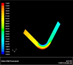 |
Fig. (3). Stress nephogram under the inlet velocity of pipe model is 2m/s. |
 |
Fig. (4). Stress nephogram under the inlet velocity of pipe model is 10m/s. |
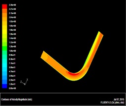 |
Fig. (5). Velocity nephogram under the inlet velocity of pipe model is 2m/s. |
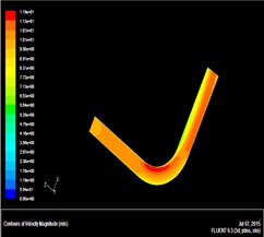 |
Fig. (6). Velocity nephogram under the inlet velocity of pipe model is 10m/s. |
From velocity nephogram, fluid velocity changes because fluid direction changes at the fluid passing the bend; from the stress nephogram, shock pressure in the bend pipe and straight pipe is not the same, the pressure in the bend pipe is obviously large. Pressure on the elbow inside wall of the lateral increases, the pressure in the inside is reduced, and the maximum stress appears in elbow inside wall of the lateral, namely pressure is the maximum at the lateral on the bend exit, next is the outside of the bent pipe head. Therefore the sensor should install on the exit of bend pipe. The sand velocity direction changed at this position, but the sand signal is still strong. Additionally, the experiment verified that the bend pipe between the sensor and noise resource can reduce the ultrasonic wave on the pipe.
3.4. Design of Matching Layer for Sand Sensor
In order to reduce the reflection of sound waves on the pipe surface, increase the effective energy of sound waves, usually it’s needed to join acoustic matching layer between transducer and working medium. Because the material of oil pipe is steel, we should use the organic glass as acoustic conductance material with easily machine shaping, little attenuation for the signal and good acoustic matching characteristics. According to the ultrasonic theory, when the ultrasonic wave shifts from one medium to another one, there will occur reflection and refraction, the theory model is shown in Fig. (7).
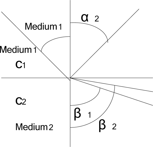 |
Fig. (7). Theory model of matching layer. |
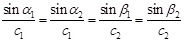
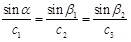
Where C1 and C2 are the velocity in the medium 1 and medium 2 respectively. Supposing the incident angle of ultrasound in medium 1 is a1, and angle of reflection is a2, angle of refraction for longitudinal wave in the medium 2 is β1, angle of refraction for transverse wave in the medium 2 is β2. According to the relation between the law of reflection and refraction:
 |
(12) |
From equation (12), a1 is equal to a2, moreover C1 is less than C2, so a1 < β1, a1 < β2 ,namely the incident angle is less than the angle of refraction.
Because the shear wave can only spread on the surface of pipe wall and internal lateral, but the wave through the pipe wall is generally longitudinal wave, so the sand signal at the interface propagates through the organic glass in the form of longitudinal wave. By the same way, the signal within the organic glass can only propagate in the form of longitudinal wave. The direction of propagation in line with the law of refraction, namely:
 |
(13) |
Because the compressional wave velocity is greater than the shear wave in the same medium, a is the incidence angle, β2 < β1 < a1 so, and β1 increases with a. When the a = 90°,
 |
(14) |
From equation (13) and (14), when β1 is larger than 27.6°, the sand signal can propagate without distortion. Considering the factors such as the degree of bending pipe wall, the angle of inclination for organic glass β1, choose 45°.
According to the literature [10], the thickness of matching layer, defined as D, which is equal to:
 |
(15) |
In this condition, the sound energy of ultrasonic sensor is largest. Where V is the sound velocity of ultrasonic wave in the steel, about 5800m/s, f is the transmission frequency, equal to 640kHz, The thickness of organic glass D can be computed from equation (15), which is about 1cm. The picture of matching layer is shown in the Fig. (8).
 |
Fig. (8). Picture of matching layer. |
4. CALIBRATION SYSTEM
4.1. Experimental Procedure
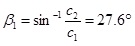
The designed sand monitoring system is shown in Fig. (9), and used to monitor the sand production. The experimental process is as follows:
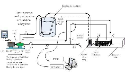 |
Fig. (9). Calibration experimental device for sand carrying ratio. |
- Mixture with oil and sand in the storage tank is injected into the pipe through the screw pump and pipe, which reflows to the recovery tank through a sand filtering net, comes into the storage tank through the submersible pump.
- Electronic scale is used to measure the sand mass, which is taken as a standard value. The sand sensor is fixed on the pipe. ISPSS and SPSAOSS should be connected correctly, which used to obtain M and U.
- While we open the sand injection port at pump inlet, sand flows into the tank.
- Before we open the pump, Un is measured when no sand pass through the pipe; then open the pump, mixture with sand flows into the pipe, then Us is measured. Using equation (10) can obtain U.
- We compute the water volume according to the tank size, measure the sand weight, compute the sand volume according to the sand density. At the same time, sand carrying ratio R is computed according to the equation (11).
- When we do experiment using sand particles with different diameter repeatedly, then can get the perfect value of K using the curve fitting method.
4.2. Experiment Result and Analysis
4.2.1. Experiment Result
When the diameter of sand particle is 20-40(mesh), Table 1 is the test result under different flow velocity with the real sand quality equal to 10g. Table 2 is the test result under different velocity with the real sand quality equal to 20g. Table 3 is the test result under different velocity with real sand quality equal to 30g.
| Velocity(m/s) | Real Value(g) | Measurement Value(g) | Measurement Error(%) |
|---|---|---|---|
| 9.3 | 10 | 1.5324 | 84.68 |
| 10.0 | 10 | 9.1921 | 8.08 |
| 13.2 | 10 | 9.6239 | 3.76 |
| 16.0 | 10 | 9.5921 | 4.08 |
| 18.1 | 10 | 9.7532 | 2.47 |
| 20.8 | 10 | 9.4134 | 5.87 |
| 23.3 | 10 | 9.5758 | 4.24 |
| 24.6 | 10 | 9.5174 | 4.83 |
| 26.7 | 10 | 9.6013 | 3.99 |
| 28.5 | 10 | 10.0862 | 0.86 |
| 30.1 | 10 | 10.0175 | 0.18 |
| 32.5 | 10 | 10.0214 | 0.21 |
| Velocity(m/s) | Real Value(g) | Measurement Value(g) | Measurement Error(%) |
|---|---|---|---|
| 9.3 | 20 | 13.1564 | 68.44 |
| 10.0 | 20 | 19.5253 | 4.75 |
| 13.2 | 20 | 19.8321 | 1.68 |
| 16.0 | 20 | 19.7531 | 2.47 |
| 18.1 | 20 | 19.7201 | 2.80 |
| 20.8 | 20 | 19.6651 | 3.35 |
| 23.3 | 20 | 19.8859 | 1.14 |
| 24.6 | 20 | 19.6573 | 3.43 |
| 26.7 | 20 | 19.7857 | 2.14 |
| 28.5 | 20 | 19.8772 | 1.23 |
| 30.1 | 20 | 20.2584 | 2.58 |
| 32.5 | 20 | 20.3426 | 3.43 |
| Velocity(m/s) | Real Value(g) | Measurement Value(g) | Measurement Error(%) |
|---|---|---|---|
| 9.3 | 30 | 24.0518 | 59.48 |
| 10.0 | 30 | 28.8543 | 11.46 |
| 13.2 | 30 | 29.6064 | 3.94 |
| 16.0 | 30 | 29.6752 | 3.25 |
| 18.1 | 30 | 29.6732 | 3.27 |
| 20.8 | 30 | 29.7843 | 2.16 |
| 23.3 | 30 | 29.7423 | 2.58 |
| 24.6 | 30 | 29.7921 | 2.08 |
| 26.7 | 30 | 29.8147 | 1.85 |
| 28.5 | 30 | 30.1724 | 1.72 |
| 30.1 | 30 | 30.1693 | 1.69 |
| 32.5 | 30 | 30.0854 | 0.85 |
From Tables 1-3, when the flow velocity is low, the measurement error between the measurement value and real value is large. The measurement error is up to 84% when the flow velocity is 9.3m/s; this means though we can measure the sand signal, but the measurement result is distorted. When the flow velocity is large than 10.0m/s, the measurement error is small, the range of measurement error is smaller than 4%.
When the diameter of sand particle is 70-140(mesh), Table 4 is the test result under different flow velocity with the real sand quality equal to 10g. Table 5 is the test result under different flow velocity with the real sand quality equal to 20g. Table 6 is the test result under different velocity with the real sand quality equal to 30g.
| Velocity(m/s) | Real Value(g) | Measurement Value(g) | Measurement Error(%) |
|---|---|---|---|
| 9.3 | 10 | 1.5319 | 84.68 |
| 10.0 | 10 | 1.5732 | 84.27 |
| 13.2 | 10 | 1.7145 | 82.86 |
| 16.0 | 10 | 9.6139 | 3.86 |
| 18.1 | 10 | 9.7741 | 2.26 |
| 20.8 | 10 | 9.7947 | 2.05 |
| 23.3 | 10 | 9.6515 | 3.49 |
| 24.6 | 10 | 9.9321 | 0.68 |
| 26.7 | 10 | 9.8765 | 1.24 |
| 28.5 | 10 | 9.6573 | 3.43 |
| 30.1 | 10 | 10.0967 | 0.97 |
| 32.5 | 10 | 10.0516 | 0.52 |
| Velocity(m/s) | Real Value(g) | Measurement Value(g) | Measurement Error(%) |
|---|---|---|---|
| 9.3 | 20 | 14.0537 | 59.46 |
| 10.0 | 20 | 15.1829 | 48.17 |
| 13.2 | 20 | 17.3925 | 26.08 |
| 16.0 | 20 | 19.6663 | 3.34 |
| 18.1 | 20 | 19.7532 | 2.47 |
| 20.8 | 20 | 19.8814 | 1.19 |
| 23.3 | 20 | 19.7561 | 2.44 |
| 24.6 | 20 | 19.9252 | 0.75 |
| 26.7 | 20 | 19.9173 | 0.83 |
| 28.5 | 20 | 19.9046 | 0.95 |
| 30.1 | 20 | 20.2235 | 2.24 |
| 32.5 | 20 | 20.3617 | 3.62 |
| Velocity(m/s) | Real Value(g) | Measurement Value(g) | Measurement Error(%) |
|---|---|---|---|
| 9.3 | 30 | 23.8721 | 61.28 |
| 10.0 | 30 | 24.9537 | 50.46 |
| 13.2 | 30 | 25.124 | 48.76 |
| 16.0 | 30 | 29.6418 | 3.58 |
| 18.1 | 30 | 29.9182 | 0.82 |
| 20.8 | 30 | 29.6561 | 3.44 |
| 23.3 | 30 | 29.6724 | 3.28 |
| 24.6 | 30 | 29.6936 | 3.06 |
| 26.7 | 30 | 29.7851 | 2.15 |
| 28.5 | 30 | 29.8013 | 1.99 |
| 30.1 | 30 | 30.0976 | 0.98 |
| 32.5 | 30 | 30.1058 | 1.06 |
From Tables 4-6, when the flow velocity is low, the error between the measurement value and real value is large. When the flow velocity is less than 13.2m/s, the measurement error is up to 61.28%.This means though we can measure the sand signal, but the measurement result is distorted. When the flow velocity is large than 16.0m/s, the measurement error is small, the range of measurement error is smaller than 4%, but the measurement value is not stable.
4.2.2. Analysis of Measurement Error
The measurement results indicated that the developed instrument could work well at the flow velocity more than 16m/s. When the flow velocity is low, the amount of sand particle striking the pipe is few, the amplitude of background noise may exceed the sand signal. Seen from the equation (9), the accumulated sand production M is small. The next research goal is to analyze how to reduce the background noise, which includes the electromagnetic interference caused by the motor, the viscosity of the oil, the vibration on the pipelines and so on. Compared to the vibration sensors, which also have low measurement accuracy on the low flow velocity, and it’s not convenient to install because the vibration sensor should be contact with the pipe directly. Also compared to the current literature, the main contribution of this paper is high measurement accuracy on the high flow velocity.
CONCLUSION AND FUTURE WORK
Compared to the current sand production monitoring system, the sand production computation model of our system is close to the characteristic of sand particle signal. And which is convenient for installing and dismantling because of using the contactless structure. The main achievements are as follows:
- The computation model for sand carrying ratio is built in the oil delivery process.
- The detection method for the sand production is given; the sand production detection system is developed.
- The calibration device of sand carrying ratio is developed, the laboratory test and field test is done.
- When the flow velocity is low, we can detect the signal, but cannot quantitatively analyze; when the flow velocity is high, the measurement result is in the 4%, and the measurement error is stable.
The measurement error of sand production is larger under low oil flow velocity. The next work is to find the source of background noise, and analyze the corresponding method to reduce the related noise; another work is to improve the sensitivity of sand sensor, which include improve the performance of matching layer and structure of whole sand sensor.
CONFLICT OF INTEREST
The authors confirm that this article content has no conflict of interest.
ACKNOWLEDGEMENTS
The authors thank the industrial technology research projects of Shaanxi Province of China (No. 2016GY-177).