RESEARCH ARTICLE
Predicting the Oil Well Production Based on Multi Expression Programming
Xin Ma*, Zhi-bin Liu
Article Information
Identifiers and Pagination:
Year: 2016Volume: 9
First Page: 21
Last Page: 32
Publisher Id: TOPEJ-9-21
DOI: 10.2174/1874834101609010021
Article History:
Received Date: 17/11/2014Revision Received Date: 03/04/2015
Acceptance Date: 26/08/2015
Electronic publication date: 9/3/2016
Collection year: 2016
open-access license: This is an open access article licensed under the terms of the Creative Commons Attribution-Non-Commercial 4.0 International Public License (CC BY-NC 4.0) (https://creativecommons.org/licenses/by-nc/4.0/legalcode), which permits unrestricted, non-commercial use, distribution and reproduction in any medium, provided the work is properly cited.
Abstract
Predicting the oil well production is very important and also quite a complex mission for the petroleum engineering. Due to its complexity, the previous empirical methods could not perform well for different kind of wells, and intelligent methods are applied to solve this problem. In this paper the multi expression programming (MEP) method has been employed to build the prediction model for oil well production, combined with the phase space reconstruction technique. The MEP has shown a better performance than the back propagation networks, gene expression programming method and the Arps decline model in the experiments, and it has also been shown that the optimal state of the MEP could be easily obtained, which could overcome the over-fitting.
1. INTRODUCTION
Prediction of oil production is very important in the petroleum industry. The prediction could help petroleum engineers to make the project decisions, adjust the current schedule, and analyze the effect of the operations, etc. However, it is difficult to predict the productions accurately, as the underground conditions are complex and full of uncertain factors, which are hard to be detected and controlled. Thus, the geological models could not be predictive when other analysis has not been contained.
Researchers found that the future production could be estimated when the historical data sets are used. The current researches could be categorized in two classes, the curve decline fitting methods and the intelligent prediction methods. The empirical equations and mathematical modeling technology are often combined to build the prediction models in the previous ones, such as the exponential, hyperbolic, and harmonic equations [1], and recent ones such as the historical matching method [2], unit proven reserve ratio method [3]. The curve fitting does not only make the matching process difficult but also results in unreliable predictions [4]. The intelligent methods, such as NDT [4], ANN [5, 6], SVM [7], have managed to fitting the data more closely, and could give more accurate results than the curve fitting ones.
However, the production forecast for one single well as the time series of oil well production follows the patterns of periodicity, seasonality, or cycle, etc. Curve fitting algorithms [8] have also been used to predict the oil well production but are limited in particular conditions. Being eligible to predict the production of the oil fields, the intelligent methods are also applied to predict the oil well production, and previous works have proved the feasibility of artificial neural network (ANN)[9-12].
Genetic algorithm(GA) is one of the state of art intelligent algorithms, which is based on the principles of the evolution theories of Darwin [13]. In the early theory of GA, the gene was encoded with decimal numbers or binary number, which made the GA failed to perform well in a plenty of complex areas.
Ferreira [14] put forward a new genetic algorithm, genetic expression programming(GEP), which encoded the gene with a binary tree that could be converted to a mathematical expression. This innovation extended the expression ability of the chromosome, and could be used for the time series prediction[15]. With its success, the GEP has been extended to multi expression programming(MEP) [16, 17]. In the MEP, individuals carried more than one gene, which means the each individual could express not only one mathematical expression but several. This extension makes the GEP more flexible and better performing.
In this paper, the prediction model based on MEP has been built, and its applicability has been evaluated. To compare the performance of MEP to previous models, the GEP, ANN and Arps decline model have also been applied to predict the oil well production in this paper.
The rest of this paper is organized as follows: Sec.2 introduces the MEP, including its relationship with the GEP; Sec.3 introduces the phase space reconstruction, which is the necessary processing when the MEP or ANN is used for time series regression, and the algorithm to build the prediction model based on MEP is summarized in Sec.4; Sec.5 presents the simulation experiment which includes the evaluation of MEP and the comparison to ANN and GEP. Conclusions are drawn in Sec.6.
2. THE MULTI EXPRESSION PROGRAMMING
2.1. Gene
Encoding the gene and constructing the chromosome could be deemed as the key criteria to distinguish different kinds of genetic algorithms. One individual only carries one gene in GEP while it carries several ones in the MEP. Being similar to the GEP, the gene is also encoded to be a mathematical expression in MEP, which could also be expressed as a binary tree. For example, in Fig. (1) there is a binary tree which contains three operators {*, +, exp} and three input parameters, where a and b are constants and x is the variable, respectively. The expression corresponding to the binary tree is (a+x)+exp(b), and such expressions are called the genes in MEP. One individual is a set of binary trees in MEP, which means a single individual contains several genes like those in Fig. (1). If one individual contains the expressions f1,f,,..fn, it will be in the form of y=a1f1+a2f2+....+anfn+b, where the, a1,a,..an, b are the parameters which will be determined by the least squares method.
In addition, the depth of the binary tree is restricted [18, 19], because if the binary tree which stands for a gene is not restricted to have a maximum depth, both the GEP and MEP will be very difficult to analyze, and the complexity will be infinite theoretically [14].
2.2. Cross Over
Cross over is actually exchanging the expression trees (or sub-trees) of each individual in order to generate new expressions. The two-point high-level operator is employed to cross over the individuals.
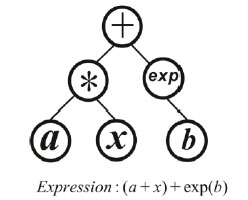 |
Fig. (1). Binary tree of the gene expression. |
Two-point means that two individuals are involved in the cross over operation. A probability will be set before the individuals are selected to be crossed over. And each time the individuals with high probability to be crossed over will be chosen, and this is what the high-level means. When two individuals have been selected to be crossed over, the genes of them will be replaced directly. Particularly, when both individuals have only one gene, they will be crossed over with the gene’s sub-trees. In this kind of situation, the cross over operation of MEP is just the same as that of GEP.
2.3. Mutation
Mutation operation is quite similar to the cross over operation. Each individual is also labeled with a probability to be mutated. And the genes which are selected to be replaced by new ones are also selected randomly, and the new genes are generated randomly with no relationship to the parent generation. This operation confirms that each generation will cabled with new structures, and the results will not be influenced by the selection of the initial conditions.
2.4. Selection
Selection is based on the evaluation of each individual. Excellent individuals could perform high-precision forecastresults in prediction problems. The index to assess the ability of prediction accuracy is the fitness, which is defined as

where theis the expected output, and theis the output of the prediction model. High fitness indicates good performance, while low fitness indicates bad performance. Each time the individuals with high fitness will be left in the next generation, while the ones with low fitness will be kicked out. Thus, the prediction results will get closer to the expected outputs by generation and generation.
3. PHASE SPACE RECONSTRUCTION
The embedded theorem of Takens [18] asserts that if the dynamical system is deterministic, the observed time series representing system can be expressed as
 |
(1) |
Where τ is the time-delay constant between samples, andis the embedded dimension. The phase space reconstruction of a set of time series
x = {x(1), x(2),...., x(n)}
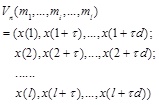
is
 |
(2) |
The reconstructed dynamic system is diffeomorphism to the original dynamic system [19], and the new system could better reflect the changing rules of the original one. Within the Eq. (2), the Eq. (1) could be converted to x(t)= f(mi). Then, the objective of regressing or predicting the time series is to find the expression of f(.). It is obviously very difficult to induce or summarize an appropriate f(.) which could perform well. But expression of f(.) could be automatically generalized by MEP. Thus, the MEP is eligible to be applied to build the prediction model of any kind of time series.
4. ALGORITHM
The algorithm to build the prediction model is summarized in Fig. (2). The time delay constant and embedded dimension will be given before reconstructing the time series data. The first generation of individuals, also the binary trees will be initialized within the given max deep of binary tree and number of genes for each individual. The best expression in each time of iteration will be stored, and the terminal expression will be chosen from all the best ones in every iteration.
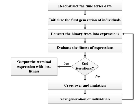 |
Fig. (2). The algorithm of building the prediction model based on MEP and phase space reconstruction. |
5. SIMULATION EXPERIMENTS
5.1. Evaluation Indices of Model Accuracy
Evaluation of the model accuracy is twofold, the fitting accuracy and the prediction accuracy. The mean square error(MSE), mean relative percentage error (MRPE), relative mean squares(RMS) and the linear correlative coefficient(R) of each model are used to compare each models performance. The numerical formulas of these indices are listed below.

 |
(3) |
5.2. RawData
The oil well selected in this paper is from one oil field of China, encoded as B52. The water cut (ratio of water production to the whole liquid production of the oil well) of this well has been above 36% since Jan, 1996, which means this oil well has entered the middle late development period. Being similar to the oil fields, the productions of oil wells also decline in the middle late development period. Fig. (3) shows the production time series of B52, and details of each point are shown in Table 1. It could be seen that the production of B52 is decreasing overall, but the production is fluctuating. 71 points of six years monthly production are used as raw data. Former 59 points are used to train the models, and last 12 points are used to test the prediction performance accuracy of each model, respectively.
 |
Fig. (3). The algorithm of building the prediction model based on MEP and phase space reconstruction. |
The monthly production data of B52.
| Time | Production | Time | Production | Time | Production | Time | Production |
|---|---|---|---|---|---|---|---|
| 1 | 38.91 | 19 | 20.19 | 37 | 2.96 | 55 | 2.24 |
| 2 | 21.3 | 20 | 14.27 | 38 | 10.64 | 56 | 1.56 |
| 3 | 19.75 | 21 | 17.31 | 39 | 17.3 | 57 | 2.79 |
| 4 | 27.82 | 22 | 19.05 | 40 | 13.12 | 58 | 1.33 |
| 5 | 9.25 | 23 | 25.87 | 41 | 14.67 | 59 | 0.52 |
| 6 | 14.29 | 24 | 7.01 | 42 | 7.84 | 60 | 4.22 |
| 7 | 19.83 | 25 | 9.37 | 43 | 4.715 | 61 | 3.73 |
| 8 | 25.97 | 26 | 12.57 | 44 | 1.59 | 62 | 3.73 |
| 9 | 22.35 | 27 | 12.2 | 45 | 3.48 | 63 | 2.59 |
| 10 | 25.67 | 28 | 12.225 | 46 | 2.15 | 64 | 1.85 |
| 11 | 15.54 | 29 | 12.25 | 47 | 1.48 | 65 | 1.85 |
| 12 | 22.49 | 30 | 8.19 | 48 | 3.34 | 66 | 2.07 |
| 13 | 21.31 | 31 | 3.69 | 49 | 4.57 | 67 | 2.04 |
| 14 | 19.38 | 32 | 7.77 | 50 | 4.45 | 68 | 5.05 |
| 15 | 25.98 | 33 | 1.03 | 51 | 4.35 | 69 | 3.89 |
| 16 | 18.35 | 34 | 6.67 | 52 | 4.22 | 70 | 6.08 |
| 17 | 26.11 | 35 | 1.48 | 53 | 2.95 | 71 | 9.18 |
| 18 | 13.76 | 36 | 1.48 | 54 | 1.85 |
Data after phase space reconstruction.
| No. | x1 | x2 | x3 | x4 | x5 | x6 | x7 | x8 | x9 | x10 | x11 | x12 | y |
|---|---|---|---|---|---|---|---|---|---|---|---|---|---|
| 1 | 38.91 | 21.30 | 19.75 | 27.82 | 9.25 | 14.29 | 19.83 | 25.97 | 22.35 | 25.67 | 15.54 | 22.49 | 21.31 |
| 2 | 21.30 | 19.75 | 27.82 | 9.25 | 14.29 | 19.83 | 25.97 | 22.35 | 25.67 | 15.54 | 22.49 | 21.31 | 19.38 |
| 3 | 19.75 | 27.82 | 9.25 | 14.29 | 19.83 | 25.97 | 22.35 | 25.67 | 15.54 | 22.49 | 21.31 | 19.38 | 25.98 |
| 4 | 27.82 | 9.25 | 14.29 | 19.83 | 25.97 | 22.35 | 25.67 | 15.54 | 22.49 | 21.31 | 19.38 | 25.98 | 18.35 |
| 5 | 9.25 | 14.29 | 19.83 | 25.97 | 22.35 | 25.67 | 15.54 | 22.49 | 21.31 | 19.38 | 25.98 | 18.35 | 26.11 |
| 6 | 14.29 | 19.83 | 25.97 | 22.35 | 25.67 | 15.54 | 22.49 | 21.31 | 19.38 | 25.98 | 18.35 | 26.11 | 13.76 |
| 7 | 19.83 | 25.97 | 22.35 | 25.67 | 15.54 | 22.49 | 21.31 | 19.38 | 25.98 | 18.35 | 26.11 | 13.76 | 20.19 |
| 8 | 25.97 | 22.35 | 25.67 | 15.54 | 22.49 | 21.31 | 19.38 | 25.98 | 18.35 | 26.11 | 13.76 | 20.19 | 14.27 |
| 9 | 22.35 | 25.67 | 15.54 | 22.49 | 21.31 | 19.38 | 25.98 | 18.35 | 26.11 | 13.76 | 20.19 | 14.27 | 17.31 |
| 10 | 25.67 | 15.54 | 22.49 | 21.31 | 19.38 | 25.98 | 18.35 | 26.11 | 13.76 | 20.19 | 14.27 | 17.31 | 19.05 |
| 11 | 15.54 | 22.49 | 21.31 | 19.38 | 25.98 | 18.35 | 26.11 | 13.76 | 20.19 | 14.27 | 17.31 | 19.05 | 25.87 |
| 12 | 22.49 | 21.31 | 19.38 | 25.98 | 18.35 | 26.11 | 13.76 | 20.19 | 14.27 | 17.31 | 19.05 | 25.87 | 7.01 |
| 13 | 21.31 | 19.38 | 25.98 | 18.35 | 26.11 | 13.76 | 20.19 | 14.27 | 17.31 | 19.05 | 25.87 | 7.01 | 9.37 |
| 14 | 19.38 | 25.98 | 18.35 | 26.11 | 13.76 | 20.19 | 14.27 | 17.31 | 19.05 | 25.87 | 7.01 | 9.37 | 12.57 |
| 15 | 25.98 | 18.35 | 26.11 | 13.76 | 20.19 | 14.27 | 17.31 | 19.05 | 25.87 | 7.01 | 9.37 | 12.57 | 12.20 |
| 16 | 18.35 | 26.11 | 13.76 | 20.19 | 14.27 | 17.31 | 19.05 | 25.87 | 7.01 | 9.37 | 12.57 | 12.20 | 12.23 |
| 17 | 26.11 | 13.76 | 20.19 | 14.27 | 17.31 | 19.05 | 25.87 | 7.01 | 9.37 | 12.57 | 12.20 | 12.23 | 12.25 |
| 18 | 13.76 | 20.19 | 14.27 | 17.31 | 19.05 | 25.87 | 7.01 | 9.37 | 12.57 | 12.20 | 12.23 | 12.25 | 8.19 |
| 19 | 20.19 | 14.27 | 17.31 | 19.05 | 25.87 | 7.01 | 9.37 | 12.57 | 12.20 | 12.23 | 12.25 | 8.19 | 3.69 |
| 20 | 14.27 | 17.31 | 19.05 | 25.87 | 7.01 | 9.37 | 12.57 | 12.20 | 12.23 | 12.25 | 8.19 | 3.69 | 7.77 |
| 21 | 17.31 | 19.05 | 25.87 | 7.01 | 9.37 | 12.57 | 12.20 | 12.23 | 12.25 | 8.19 | 3.69 | 7.77 | 1.03 |
| 22 | 19.05 | 25.87 | 7.01 | 9.37 | 12.57 | 12.20 | 12.23 | 12.25 | 8.19 | 3.69 | 7.77 | 1.03 | 6.67 |
| 23 | 25.87 | 7.01 | 9.37 | 12.57 | 12.20 | 12.23 | 12.25 | 8.19 | 3.69 | 7.77 | 1.03 | 6.67 | 1.48 |
| 24 | 7.01 | 9.37 | 12.57 | 12.20 | 12.23 | 12.25 | 8.19 | 3.69 | 7.77 | 1.03 | 6.67 | 1.48 | 1.48 |
| 25 | 9.37 | 12.57 | 12.20 | 12.23 | 12.25 | 8.19 | 3.69 | 7.77 | 1.03 | 6.67 | 1.48 | 1.48 | 2.96 |
| 26 | 12.57 | 12.20 | 12.23 | 12.25 | 8.19 | 3.69 | 7.77 | 1.03 | 6.67 | 1.48 | 1.48 | 2.96 | 10.64 |
| 27 | 12.20 | 12.23 | 12.25 | 8.19 | 3.69 | 7.77 | 1.03 | 6.67 | 1.48 | 1.48 | 2.96 | 10.64 | 17.30 |
| 28 | 12.23 | 12.25 | 8.19 | 3.69 | 7.77 | 1.03 | 6.67 | 1.48 | 1.48 | 2.96 | 10.64 | 17.30 | 13.12 |
| 29 | 12.25 | 8.19 | 3.69 | 7.77 | 1.03 | 6.67 | 1.48 | 1.48 | 2.96 | 10.64 | 17.30 | 13.12 | 14.67 |
| 30 | 8.19 | 3.69 | 7.77 | 1.03 | 6.67 | 1.48 | 1.48 | 2.96 | 10.64 | 17.30 | 13.12 | 14.67 | 7.84 |
| 31 | 3.69 | 7.77 | 1.03 | 6.67 | 1.48 | 1.48 | 2.96 | 10.64 | 17.30 | 13.12 | 14.67 | 7.84 | 4.72 |
| 32 | 7.77 | 1.03 | 6.67 | 1.48 | 1.48 | 2.96 | 10.64 | 17.30 | 13.12 | 14.67 | 7.84 | 4.72 | 1.59 |
| 33 | 1.03 | 6.67 | 1.48 | 1.48 | 2.96 | 10.64 | 17.30 | 13.12 | 14.67 | 7.84 | 4.72 | 1.59 | 3.48 |
| 34 | 6.67 | 1.48 | 1.48 | 2.96 | 10.64 | 17.30 | 13.12 | 14.67 | 7.84 | 4.72 | 1.59 | 3.48 | 2.15 |
| 35 | 1.48 | 1.48 | 2.96 | 10.64 | 17.30 | 13.12 | 14.67 | 7.84 | 4.72 | 1.59 | 3.48 | 2.15 | 1.48 |
| 36 | 1.48 | 2.96 | 10.64 | 17.30 | 13.12 | 14.67 | 7.84 | 4.72 | 1.59 | 3.48 | 2.15 | 1.48 | 3.34 |
| 37 | 2.96 | 10.64 | 17.30 | 13.12 | 14.67 | 7.84 | 4.72 | 1.59 | 3.48 | 2.15 | 1.48 | 3.34 | 4.57 |
| 38 | 10.64 | 17.30 | 13.12 | 14.67 | 7.84 | 4.72 | 1.59 | 3.48 | 2.15 | 1.48 | 3.34 | 4.57 | 4.45 |
| 39 | 17.30 | 13.12 | 14.67 | 7.84 | 4.72 | 1.59 | 3.48 | 2.15 | 1.48 | 3.34 | 4.57 | 4.45 | 4.35 |
| 40 | 13.12 | 14.67 | 7.84 | 4.72 | 1.59 | 3.48 | 2.15 | 1.48 | 3.34 | 4.57 | 4.45 | 4.35 | 4.22 |
Data after phase space reconstruction.
| No. | x1 | x2 | x3 | x4 | x5 | x6 | x7 | x8 | x9 | x10 | x11 | x12 | y |
|---|---|---|---|---|---|---|---|---|---|---|---|---|---|
| 41 | 14.67 | 7.84 | 4.72 | 1.59 | 3.48 | 2.15 | 1.48 | 3.34 | 4.57 | 4.45 | 4.35 | 4.22 | 2.95 |
| 42 | 7.84 | 4.72 | 1.59 | 3.48 | 2.15 | 1.48 | 3.34 | 4.57 | 4.45 | 4.35 | 4.22 | 2.95 | 1.85 |
| 43 | 4.72 | 1.59 | 3.48 | 2.15 | 1.48 | 3.34 | 4.57 | 4.45 | 4.35 | 4.22 | 2.95 | 1.85 | 2.24 |
| 44 | 1.59 | 3.48 | 2.15 | 1.48 | 3.34 | 4.57 | 4.45 | 4.35 | 4.22 | 2.95 | 1.85 | 2.24 | 1.56 |
| 45 | 3.48 | 2.15 | 1.48 | 3.34 | 4.57 | 4.45 | 4.35 | 4.22 | 2.95 | 1.85 | 2.24 | 1.56 | 2.79 |
| 46 | 2.15 | 1.48 | 3.34 | 4.57 | 4.45 | 4.35 | 4.22 | 2.95 | 1.85 | 2.24 | 1.56 | 2.79 | 1.33 |
| 47 | 1.48 | 3.34 | 4.57 | 4.45 | 4.35 | 4.22 | 2.95 | 1.85 | 2.24 | 1.56 | 2.79 | 1.33 | 0.52 |
| 48 | 3.34 | 4.57 | 4.45 | 4.35 | 4.22 | 2.95 | 1.85 | 2.24 | 1.56 | 2.79 | 1.33 | 0.52 | 4.22 |
| 49 | 4.57 | 4.45 | 4.35 | 4.22 | 2.95 | 1.85 | 2.24 | 1.56 | 2.79 | 1.33 | 0.52 | 4.22 | 3.73 |
| 50 | 4.45 | 4.35 | 4.22 | 2.95 | 1.85 | 2.24 | 1.56 | 2.79 | 1.33 | 0.52 | 4.22 | 3.73 | 3.73 |
| 51 | 4.35 | 4.22 | 2.95 | 1.85 | 2.24 | 1.56 | 2.79 | 1.33 | 0.52 | 4.22 | 3.73 | 3.73 | 2.59 |
| 52 | 4.22 | 2.95 | 1.85 | 2.24 | 1.56 | 2.79 | 1.33 | 0.52 | 4.22 | 3.73 | 3.73 | 2.59 | 1.85 |
| 53 | 2.95 | 1.85 | 2.24 | 1.56 | 2.79 | 1.33 | 0.52 | 4.22 | 3.73 | 3.73 | 2.59 | 1.85 | 1.85 |
| 54 | 1.85 | 2.24 | 1.56 | 2.79 | 1.33 | 0.52 | 4.22 | 3.73 | 3.73 | 2.59 | 1.85 | 1.85 | 2.07 |
| 55 | 2.24 | 1.56 | 2.79 | 1.33 | 0.52 | 4.22 | 3.73 | 3.73 | 2.59 | 1.85 | 1.85 | 2.07 | 2.04 |
| 56 | 1.56 | 2.79 | 1.33 | 0.52 | 4.22 | 3.73 | 3.73 | 2.59 | 1.85 | 1.85 | 2.07 | 2.04 | 5.05 |
| 57 | 2.79 | 1.33 | 0.52 | 4.22 | 3.73 | 3.73 | 2.59 | 1.85 | 1.85 | 2.07 | 2.04 | 5.05 | 3.89 |
| 58 | 1.33 | 0.52 | 4.22 | 3.73 | 3.73 | 2.59 | 1.85 | 1.85 | 2.07 | 2.04 | 5.05 | 3.89 | 6.08 |
| 59 | 0.52 | 4.22 | 3.73 | 3.73 | 2.59 | 1.85 | 1.85 | 2.07 | 2.04 | 5.05 | 3.89 | 6.08 | 9.18 |
Evaluation indices results of fitting of different models.
| GEP | ANN | Arps | MEP | |
|---|---|---|---|---|
| MSE | 12.7578 | 0.0772 | 30.6284 | 10.6650 |
| RMS | 3.5718 | 0.2779 | 5.5343 | 3.2657 |
| MRPE(%) | 57.8088 | 5.3862 | 70.9904 | 60.0262 |
| R | 0.8824 | 0.9993 | 0.8150 | 0.9009 |
Evaluation indices results of fitting of different models.
| GEP | ANN | Arps | MEP | |
|---|---|---|---|---|
| MSE | 4.1131 | 8.4920 | 7.6548 | 3.2877 |
| RMS | 2.0281 | 2.9141 | 2.7667 | 1.8132 |
| MRPE(%) | 26.9855 | 49.3731 | 34.9134 | 30.6310 |
| R | 0.6607 | 0.3839 | -0.4807 | 0.5893 |
Fitting evaluation indices of MEP with different genes.
| Max Genes | MSE | RMS | MRPE (%) | R |
|---|---|---|---|---|
| 2 | 10.6650 | 3.2657 | 60.0262 | 0.9009 |
| 3 | 6.1899 | 2.4880 | 51.2256 | 0.9437 |
| 4 | 7.6679 | 2.7691 | 47.0716 | 0.9297 |
| 5 | 5.9073 | 2.4305 | 52.3393 | 0.9463 |
| 6 | 4.8090 | 2.1930 | 46.0785 | 0.9565 |
| 7 | 5.6145 | 2.3695 | 50.2911 | 0.9491 |
| 8 | 3.1234 | 1.7673 | 38.3606 | 0.9720 |
| 9 | 3.2368 | 1.7991 | 37.8626 | 0.9710 |
| 10 | 4.0200 | 2.0050 | 37.2602 | 0.9638 |
Prediction evaluation indices of MEP with different genes.
| Max Genes | MSE | RMS | MRPE (%) | R |
|---|---|---|---|---|
| 2 | 3.2877 | 1.8132 | 30.6310 | 0.5893 |
| 3 | 3.2265 | 1.7962 | 29.3161 | 0.5900 |
| 4 | 5.6669 | 2.3805 | 27.7666 | 0.4904 |
| 5 | 2.9651 | 1.7219 | 44.5286 | 0.5742 |
| 6 | 3.3259 | 1.8237 | 26.5876 | 0.7020 |
| 7 | 4.1276 | 2.0317 | 31.5460 | 0.5714 |
| 8 | 4.2060 | 2.0509 | 36.7593 | 0.4223 |
| 9 | 4.5620 | 2.1359 | 41.9879 | 0.5564 |
| 10 | 4.9292 | 2.2202 | 45.5722 | 0.5202 |
5.3. Experiment 1: Compared to ANN and GEP
The time delay constantis set as 1, and the embedded dimensionis set as 12, respectively. Data after phase space reconstruction is shown in Table 2a and Table 2b, of which the first 47 points are used to build the ANN, GEP and MEP models, where x1, x2, x3...,x12 for input and y for output, respectively.
The ANN and GEP are all coded by C# from the open source project Aforge. NET [20], and the platform is Visual Studio 2010. MEP is from the updated MEP tool box GPTIPS [17], which has been updated in August 2013. The max gene tree length is 5, population is 100, and generations are 100 of both the GEP and MEP. Each GEP individual only carries one gene and each MEP individual carries 2 genes for most. The terminal expression of MEP is shown below
 |
(4) |
The MEP is also compared to the typical back propagation network(BP-ANN) in this experiment. The ANN has been show a very strong ability of fitting in a plenty of researches, but over fitting often occurred in a lot of fields, including this experiment.
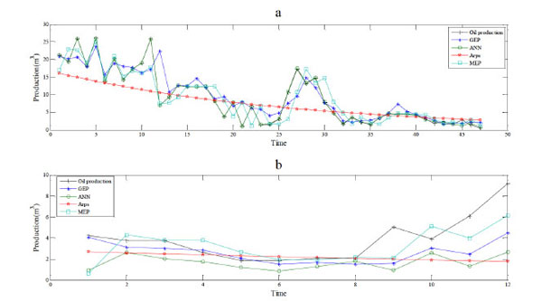 |
Fig. (4). The algorithm of building the prediction model based on MEP and phase space reconstruction. |
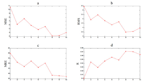 |
Fig. (5). The algorithm of building the prediction model based on MEP and phase space reconstruction. |
The fitting effect gets better when iterations increase, but meanwhile the prediction accuracy gets lower. The balance of fitting and prediction accuracy is found at 5000 times of iteration. The Arps decline model has also been used for comparison, three typical decline curves in Arps model, including the exponential decline, harmonic decline and hyperbolic decline curve, have been applied, and the raw data in this experiment shows the characteristic of exponential decline.
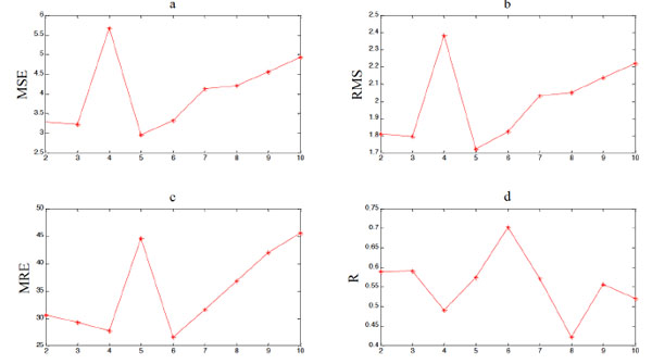 |
Fig. (6). The algorithm of building the prediction model based on MEP and phase space reconstruction. |
Simulation results are shown in Fig. (4), and evaluation indices of fitting and prediction are shown in Table 3 and Table 4, respectively. Obviously, the ANN shows the best fitting performance but the worst prediction performance. The Arps model performs worst in fitting and worse than the GEP and MEP in prediction. This indicates the genetic programming models are more eligible to build the prediction models. The MEP shows a better performance of fitting, and similar performance ofprediction to the GEP. And higher fitting precision of MEP indicates that more genes lead to more powerful ability of expression for gene expression programming models.
5.4. Experiment 2: Comparison of Different Number of Genes
MEP models with different number of genes have also been tested, and results are shown in Table 5, Table 6 and Fig. (5), Fig. (6), and the Matlab code of expressions with different number of genes is shown in the Appendix. It is shown that more genes lead to better fitting performance of MEP overall. But the prediction performance persists to get worse after the maximum genes exceed 5, which indicates the risk of over fitting still exists. Thus, when the MEP is employed to build a prediction model, the number of maximum genes should be restricted. And it is not hard to find out the optimal one by simulation experiments. Obviously, in this experiment, the optimal number of maximum genes is 6.
CONCLUSION
The multi expression programming algorithm has been applied to build the prediction model for oil well. As each individual carries several genes, the MEP has a more powerful ability of expression than the GEP. It has been shown in the experiment the MEP performed much better than the BP-ANN in predicting the oil well production even with less iterations. And also the MEP has shown a better performance than the Arps model.
Over-fitting would also occur to the MEP, nevertheless, it is easy to find an optimal number of maximum genes of the MEP, which could guarantee the MEP an optimal fitting and prediction performance. Thus, the MEP is eligible to build the production prediction model for oil well, which is better than the previous intelligent methods.
APPENDIX
The Matlab code for the expressions of MEP with different maximum genes is shown as follows, which can be directly run in the Matlab(versions after 7.0) platform. In these expressions the variable x is a matrix which stores the input data like it in Table 2(a) and Table 2(b).
Expression with 2 Genes:
y=1.001.*x(:,12)+1.539.*10.^(-8).*x(:,11).*x(:,12).^2.*x(:,2).*x(:,6).*(x(:,12)-0.9226).*(x(:,11)-x(:,12))+0.06974;
Expression with 3 Genes:
y=0.6072.*x(:,12)+0.1518.*x(:,2)-0.1518.*x(:,8)+6.725.*10.^(-6).*(x(:,11)-1.78.*x(:,5)).*(x(:,8)-x(:,12).*(x(:,12)-x(:,7))).*(-x(:,12).^2+x(:,5)+x(:,8))+1.808.*10.^(-6).*x(:,11).*x(:,4).*x(:,8).^2.*(x(:,11)-1.679)+1.22;
Expression with 4 Genes:
y=0.2352.*x(:,12)-0.2352.*x(:,11)-0.01598.*x(:,10)+0.2352.*x(:,2)-0.01598.*x(:,11).*x(:,12)+0.0002265.*x(:,11).*(x(:,10)-x(:,9))+0.007992.*x(:,11).*x(:,12).^2-0.0002265.*x(:,11).*x(:,12).^3+1.254.*10.^(-6).*x(:,11).*x(:,2).*(x(:,10).*x(:,11)+x(:,11).*x(:,2))+0.0002265.*x(:,11).*x(:,7).*(x(:,10)-x(:,9))-1.254.*10.^(-6).*x(:,11).*x(:,12).^2.*x(:,2).*(2.975.*x(:,12)-1.474.*x(:,7))+1.5;
Expression with 5 Genes:
y=0.8499.*x(:,12)-0.3188.*x(:,10)-0.09604.*x(:,1)+0.09731.*x(:,2)-0.0743.*x(:,3)+0.2554.*x(:,4)-0.2554.*x(:,6)-0.001273.*x(:,6).*(1.009.*x(:,12)-x(:,10).*x(:,7))+5.026.*10.^(-6).*x(:,12).*x(:,6).*(x(:,12)-7.029).*(x(:,11)-x(:,12)).*(2.*x(:,12)-x(:,1)+7.289)+2.308;
Expression with 6 Genes:
y=0.003414.*(x(:,12)-x(:,6)).*(x(:,12).*x(:,4)-x(:,11).*x(:,8))-0.01387.*x(:,11).*x(:,7)-0.0001618.*x(:,12).^2.*(x(:,12).^2+x(:,11)+x(:,7))+0.0001148.*(5.016.*x(:,6)+x(:,11).*x(:,7)).*(x(:,12).^2+x(:,7)-5.016.*x(:,8)+9.749)+0.07503.*x(:,12).^2+0.01009.*x(:,4).^2+2.037;
Expression with 7 Genes:
y=0.7615.*x(:,12)-0.0002035.*x(:,1)+0.2133.*x(:,2)+7.968.*10.^(-5).*x(:,5)-0.1825.*x(:,7)-0.01572.*(x(:,11)+2.065).*(x(:,5)-x(:,6))+7.968.*10.^(-5).*x(:,5).*x(:,8)-1.32.*10.^(-6).*x(:,12).^3.*x(:,2).*(x(:,5)-x(:,7)+x(:,9)-3.547)-7.968.*10.^(-5).*x(:,11).*x(:,12).*(x(:,2)+x(:,5)).*(x(:,6)-x(:,1)+11.75)+0.0002035.*x(:,11).*x(:,5).*x(:,7).*(x(:,6)-x(:,1)+11.75)+0.178;
Expression with 8 Genes:
y=0.04032.*x(:,4)-0.06543.*x(:,5)+0.198.*x(:,9)+0.006761.*(x(:,1)+x(:,5)).*(x(:,2)+x(:,4)+x(:,7)-x(:,8)-8.61)-0.02511.*x(:,10).*x(:,9)-0.007159.*x(:,3).*(x(:,2)-x(:,4))+0.007159.*x(:,3).*(x(:,4)-x(:,6))+0.007159.*(3.02.*x(:,12)-2.*x(:,5)).*(2.*x(:,12)+x(:,4)+6.522)+6.741.*10.^(-5).*(x(:,4)-x(:,1).*x(:,12)+x(:,12).*x(:,9)+x(:,5).*x(:,8)).*(x(:,10)+2.*x(:,12)-x(:,7)+x(:,5).*x(:,6))-4.621.*10.^(-5).*x(:,12).*x(:,9).*(3.02.*x(:,12)-2.*x(:,5)+x(:,11).*x(:,5))+0.0001131.*x(:,12).*(x(:,2)-8.61).*(x(:,12)-x(:,7)).*(x(:,12)+x(:,2)-x(:,10).*(x(:,12)+x(:,3))+8.61)+9.806.*10.^(-5).*x(:,12).*(x(:,2)-8.61).*(x(:,12)-x(:,7)).*(x(:,9)-x(:,12)+x(:,10).*(x(:,12)+x(:,3)))+2.326;
Expression with 9 Genes:
y=0.7413.*x(:,12)-0.08516.*x(:,3)+1.11.*x(:,6)-0.08516.*x(:,9)-0.1703.*x(:,6).*x(:,7)-6.023.*10.^(-5).*(x(:,8).*(x(:,3)-6.195)-x(:,3).^2.*(x(:,6)-2.805)).*(x(:,9)-8.971)-0.0001469.*x(:,5).*(2.*x(:,12)+x(:,6))-0.001912.*x(:,7).^2.*(x(:,12)-6.714)+0.007048.*x(:,6).*x(:,7).^2-0.0001936.*(x(:,12).*x(:,5)-6.714).*(x(:,12)-6.714).*(x(:,2)-x(:,7))+0.0001469.*x(:,1).*x(:,10).*x(:,7).*(x(:,2)-x(:,7))+0.0003981.*(x(:,3)+x(:,9)).*(x(:,12)-6.714).*(x(:,12)-x(:,4)).*(x(:,2)-x(:,8))-1.164;
Expression with 10 Genes:
y=0.006664.*x(:,1)-0.4872.*x(:,10)+0.0067.*x(:,11)+1.283.*x(:,12)+0.4717.*x(:,2)+0.2336.*x(:,4)-0.2283.*x(:,5)+0.001464.*x(:,6)+3.604.*10.^(-5).*x(:,8)+0.0001917.*(x(:,3).^2+x(:,6).*x(:,8)).*(x(:,1)+x(:,11)+x(:,5)+5.496)-3.604.*10.^(-5).*(x(:,6)+1.609).*(x(:,2)-x(:,4))-3.604.*10.^(-5).*x(:,3).*x(:,4)+0.001093.*(x(:,2).*x(:,3)+x(:,10).*x(:,6)).*(x(:,10)-x(:,2)-x(:,3)+x(:,7))+0.009392.*(x(:,10)-x(:,2)).*(x(:,12)-x(:,3)-x(:,5)+x(:,7)+5.496)-0.02338.*x(:,5).*(x(:,1)-x(:,9))-0.001464.*x(:,12).^3-3.604.*10.^(-5).*(x(:,11)+x(:,5)).*(x(:,4)+x(:,9)).*(x(:,7)+x(:,8)+x(:,9))-1.13;
CONFLICT OF INTEREST
The authors confirm that this article content has no conflict of interest.
ACKNOWLEDGEMENTs
The authors thank the editors and anonymous referees for their useful comments and suggestions, which have helped to improve this paper. This research was supported by the natural fund of education department of Sichuan Province (No.14ZB0388), the China Postdoctoral Science Foundation funded project, No:2014M562509XB, and the Scientific Project of Sichuan Provincial Education Department (No. 15ZB0447).
REFERENCES
| [1] | Kewen L, Horne RN. A Decline Curve Analysis Model Based on Fluid Flow Mechanisms. In: SPE Western Regional/AAPG Pacific Section Joint Meeting, May 19-24, 2003. California: USA 2003; pp. 1-35. |
| [2] | Fengde Z. History matching and production prediction of a horizontal coalbed methane well. J Petrol Sci Eng 2012; 96: 22-36. |
| [3] | Charpentier RR, Cook TA. Improved USGS Methodology For Assessing Continuous Petroleum Resources 2010. |
| [4] | Li X, Chan CW, Nguyen HH. Application of the neural decision tree approach for prediction of petroleum production. J Petrol Sci Eng 2013; 104: 11-6. |
| [5] | Banbi AH, Wattenbarge RA. Analysis of commingled tight gas reservoirs In: In: SPE Annual Technical Conference and Exhibition. Society of Petroleum Engineers 1996; pp. 545-55. |
| [6] | Nguyen HH, Chan CW, Wilson M. Prediction of oil well production: A multiple-neural-network approach. Intell Data Anal 2004; 8: 183-96. |
| [7] | Zhong Y, Zhao L, Liu Z, Xu Y, Li R. Using a support vector machine method to predict the development indices of very high water cut oilfields. Pet Sci 2010; 7: 379-84. |
| [8] | Ma X, Luo D, Ding XF, Zhou J. An algorithm based on the GM (1, 1) model on increasing oil production of measures operation for a single well In: International Conference on Grey Systems and Intelligent Services; Macao: China: 2013; pp. 158-60. |
| [9] | Schrader , Mary S, Balch RS, Ruan T. Using neural networks to estimate monthly production: a case study for the devonian carbonates southeast new Mexico In: SPE Production Operations Symposium, April 16-19. Okalhama City: Okalhama 2005. |
| [10] | Bansal Y, Ertekin T, Karpyn Z, et al. Forecasting well performance in a discontinuous tight oil reservoir using artificial neural networks. In: SPE Unconventional Resources Conference-USA, April 10-12. Texas: USA 2013. |
| [11] | Menezes JP, Barreto GA. Long-term time series prediction with the NARX network: an empirical evaluation. Neurocomputing 2008; 71: 3335-43. |
| [12] | Holland JH. Adaptation in Natural and Artificial Systems: an Introductory Analysis with Applications to Biology, Control, and Artificial Intelligence. USA: Michigan Press 1975. |
| [13] | Zhiyuan G, Wang Y, Liu Q. Genetic algorithms based on bintree structure encoding. J Tsinghua Univ 2000; 10: 125-8. |
| [14] | Ferreira C. Function Finding and the Creation of Numerical Constants in Gene Expression Programming. In: Advances in Soft Computing. London: Springer 2003; pp. 257-65. |
| [15] | Lopes HS, Wagner WR. A gene expression programming system for time series modeling In: Proceedings of XXV Iberian Latin American Congress on Computational Methods in Engineering (CILAMCE), November 10-12, 2004. Brazil: Recife 2004. |
| [16] | Mihai O, Dumitrescu D. Multi Expression Programming 2002. Tech. Report UBB-01-2002, Babes-Bolyai Uni.: Cluj-Napoca, Romania, 2002. |
| [17] | Searson DP, Leahy DE, Willis MJ. GPTIPS: an open source genetic programming toolbox for multigene symbolic regression In: Proceedings of the International Multiconference of Engineers and Computer Scientist, March 17-19, 2010. Hong Kong. 2010; 1: pp. 77-80. |
| [18] | Takens F. Detecting strange attractors in turbulence. Lect Notes Math 1981; 898: 366-81. |
| [19] | Tim S, Yorke JA, Casdagli M. Embedology. J Stat Phys 1991; 65: 579-616. |
| [20] | Kirillo A. CODE PROJECT, AForge.NET Open Source Framework Available from: http://www.codeproject.com/Articles/16859/ AForge-NET-open-source-framework |


