
RESEARCH ARTICLE
Mechanisms for Controlling Sand-Induced Corrosion in Horizontal Pipe Flow of Sand, Crude Oil and Water
Samuel Eshorame Sanni*, Sam Sunday Adefila, Ambrose Nwora Anozie, Oluranti Agboola
Article Information

Identifiers and Pagination:
Year: 2017Volume: 10
First Page: 220
Last Page: 238
Publisher Id: TOPEJ-10-220
DOI: 10.2174/1874834101710010220
Article History:
Received Date: 13/03/2017Revision Received Date: 31/07/2017
Acceptance Date: 31/08/2017
Electronic publication date: 16/10/2017
Collection year: 2017
open-access license: This is an open access article distributed under the terms of the Creative Commons Attribution 4.0 International Public License (CC-BY 4.0), a copy of which is available at: https://creativecommons.org/licenses/by/4.0/legalcode. This license permits unrestricted use, distribution, and reproduction in any medium, provided the original author and source are credited.
Abstract
Background:
The presence of sand particles and associated water in crude oil calls for serious concern when the flow conditions leading to flow stratification in an upstream petroleum pipeline become significant. At such conditions, problems such as sand deposition and water containment on the pipe wall may result in consequences such as sand-induced corrosion, mechanical failure, pipe fatigue, reduced flow area, loss of production and pipe blockage which are still currently unresolved by conventional and current models.
Objective:
A modelling approach was adopted to control the conditions leading to sand-induced corrosion and other related problems caused by flow stratification in the upstream petroleum sector since conventional methods adopted to screen sand, only contribute to the problem. Also, to date, mechanisms and models exist for other corrosion types such as CO2, H2S, acid-induced corrosion, etc. but none currently exists for sand-induced corrosion. However, the concept of force-competition or dimensionless numbers was adopted using a modelling approach to resolve the problem.
Method:
This research work resolves the situation by means of a three-phase model which incorporates sand, crude oil and water phases in its mass and momentum balance equations while taking into cognisance, the effect of eddies. The three-layer model established in this work, has its origin in a two-phase sand-crude oil system and, based on current literature, a modelling approach that considers the flow of sand, crude oil and water has never been adopted to tackle the problem of sand-induced corrosion caused by associated water as a stimulant for corrosion.
Conclusion:
The established model gave an accuracy of 99% when results from the model were compared with sand and crude oil production data obtained from the field. Based on the model’s reliability, flow mechanisms/dimensionless numbers were used to ascertain critical flow conditions in order to be able to avoid situations leading to sand deposition, sand-induced corrosion and other related problems. Based on the results obtained, the estimated Euler numbers revealed that the 18 m point of the pipe is at risk due to the impact of the sand-deposit-drag-force on the pipe wall. Also, the estimated Froude numbers were indicative of the 12-18 m points as deposit/corrosion prone areas.
1. INTRODUCTION
Many pipe flow scenarios are characterized by the components that make up the systems. Upstream petroleum fluids are often known to comprise of three components such as sand, crude oil and water or four components namely sand, gas, crude oil and water which must be transported to the well heads from reservoirs for further action. Adeyanju and Oyekunle [1] developed a model for predicting the bottom hole pressure of a well. Their model gave good performance with higher levels of accuracy because of its ability to incorporate the onset and influence of sanding/sand drag on the flow velocity of the flowing stream which in turn results in higher fluid viscosities and pressure drop than could be obtained with previously established models. Berrone and Marro [2] carried out space time adaptive simulations of the problems associated with laminar flow. The problems were resolved using the Navier Stoke’s equations for steady and unsteady state conditions. Boulanger and Wong [3] carried out an experimental study of the situations leading to sand deposition for sand slurry suspension in a horizontal transparent pipe loop system; they established and determined two important velocities namely, the sand deposition and the minimum sand transport velocities. Chu et al. [4] applied a two-way coupled Computational Flow Dynamics (CFD) and Discrete Element Model (DEM) to a multiphase flow scenario of a mixture of air, water and fines of magnetite with their movements and interactions determined using the Navier Stoke’s and Newton’s equations; and found that at low fluctuations/flow rates within a region of the cyclone, particles settling under gravitational influence did so at longer residence time. Darvazani et al. [5] carried out an experimental investigation of the effective and thermo-diffusion coefficients of helium-nitrogen and helium-carbon dioxide gaseous mixtures through porous cylindrical containers filled with glass spheres. They applied the transient state method in estimating the thermos-diffusion and Fick’s coefficient of diffusion; the model predictions were in agreement with experimental measurements. Simulation of laminar flow of sand and crude oil in a horizontal oil well has been modelled [6], however, the model cannot handle situations involving turbulent flows. Giveler and Mikataranian [7] gave correlations for determining friction factor and Reynold’s number of a particle in laminar and turbulent flows. Other works on multiphase flows have their various applications some of which include the works of Horender and Hardalupas [8] who carried out vortex simulations of a two-phase dilute particle laden system to determine the correlation between fluid-particle motion and the transfer of turbulent kinetic energy between both phases. From their findings, the particles Stoke’s number was influenced by the particle concentration and slip between both phases. Also, the particles showed reduced fluctuations due to the particle concentration/population at a given point. Flow operators are sometimes faced with transport challenges including: sand deposition, slugging, partial pipe blockage, corrosion, abrasion, mechanical wear, reduction of efficiency, low oil recovery from the lines and well shut down [9], when a mixture comprising the aforementioned challenges is to be transported from the well bore to the well head.
In this work, the flow of sand, crude oil and water in a horizontal pipeline was considered in order to be able to describe adequately and accurately, by means of a model, the force competitions or interactions taking place in the system. A study was carried out on thixotropic interparticle interactions of silica and non-ionic polymeric particles in an aqueous medium [10]. Based on their findings, the obtained results compared favourably with published literature on the subject. Liu et al. [11] carried out a numerical simulation of the Reynold’s stress on the interactions in a gas-particle binary system. The results showed that the Reynolds stress near the walls and at the concentric region were responsible for the stratified flow, that is, it was higher at the walls than in the concentric region of the pipe. The review of Rahmati et al. [12] on sand prediction models asserts that numerical and analytical sand transport models have some measured degree of success in quantifying and determining the amount of sand and the onset of sanding in reservoirs but are deficient in predicting sand mass and rate of sanding in petroleum reservoirs, hence there is a need to improve the existing models and technologies. Flow directions are often influenced by forces which provide insight into the prevailing force mechanisms responsible for transport. When the surface of the reservoir fluid at the well bore is sheared, the inertia forces tend to distort the interfacial tension thus, the fluid gains momentum and is given a lift off the formation zone. The mixture then flows through perforations into the oil well lined with pipes through which the reservoir fluid flows.
The mechanisms considered here are inertia forces, viscous forces, momentum diffusivity, molecular diffusivity, gravity and pressure forces [6, 13, 14]. Particle deposition in fluid-solid systems result from pressure drops where the system becomes stratified with the different layers experiencing interfacial force and pressure effects [15]. Numerical simulations of the two phase flow in a particle-laden channel were carried out by Wang [16]. Streaky and cloudy orientations of particles in the stream were known to be weakened by increased inertia forces. Turbulence modulation increased with particle loading at the walls and reduced as particle concentration dropped. Zhou et al. [17] carried out the numerical simulation of a shale-shaker/vibration equipment for screening sand during the transport of petroleum fluid. The particle trajectory was simulated using the discrete element method and it was asserted that particle size has a great influence on its transport velocity and the particle filter ratio is a function of the screen vibration frequency.
In order to solve the problem of sand-induced corrosion of petroleum pipes caused by flow stratification resulting from sand deposition and water accumulation in the lines, there is need to look beyond the already existing fluid-particle models or multiphase flow models in the bid to establish an appropriate model for determining the conditions that can cause sand-induced corrosion or mechanical wear of petroleum pipelines. This is because, although the models discussed were established for fluid-particle systems, none of the works cited and those of current literature on the subject have established a model approach to tackle the problem of sand-induced corrosion of petroleum pipes which centres on using the concept of dimensionless numbers alongside the incorporation of sand, water and crude oil concentration and velocity terms.
Previously established models are for other particulate/sand and water, air/gas systems but there is no model describing the flow scenario in a crude oil-sand-water system in relation to sand-induced corrosion and deposition mechanisms. Also, the Reynold’s number is the most popularly discussed mechanism without emphasis on other important flow mechanisms such as momentum and molecular diffusivities, Froude and Euler numbers.
2. DATA COLLECTION
Field data was generated using flow facilities set up by ADDAX Petroleum in Owerri, Imo state, Nigeria. Reservoir fluid was introduced into the well line (that is, 78 ft; 24 m pipeline) by means of a pump situated at the well bore which links the wellbore to the flowing tubing head. The line had three integrated sand screens/filters located at the suction, 8 and 14 m points of the pipe which helped to remove coarse, medium sized and fine sand particles respectively. A Supervisory Computer-Aided Data Acquisition Machine was used to obtain data from the producing well. The produced sand, water and crude oil Feeder lines were then used to transport the fluid to a separator from which the amount of crude oil, water and sand were determined. Sand particles hardness (that is, average particle hardness = 800 Vickers) was determined using a pyknometer. The data obtained from flow measurements are as indicated in Table 1.
| Choke (-) | FTP (psia) | API (o) | GAS (scf/d) | BSW (%) | BLPD (bbl/d) | BOPD (bbl/d) | GOR (-) | Pinj (psia) | GL rate (scf/d) | Sand PTB (lb/bbl) |
|---|---|---|---|---|---|---|---|---|---|---|
| 44 | 793 | 20.3 | 2293 | 47 | 2502 | 1326 | 1729 | 1100 | 540 | 1.22 |
| 44 | 748 | 20.6 | 2148 | 46.5 | 2342 | 1254 | 1714 | 1120 | 402 | 1.31 |
| 44 | 550 | 20.8 | 681 | 45 | 1797 | 988 | 689 | 1220 | 420 | 1.31 |
| 44 | 760 | 20.8 | 649 | 47 | 2198 | 1165 | 557 | 1220 | 550 | 1.31 |
| 44 | 700 | 20.5 | 2161 | 50.3 | 2293 | 1140 | 1896 | 1200 | 386 | 2.55 |
| 44 | 800 | 20.6 | 3183 | 50 | 2375 | 1188 | 2680 | 1206 | 316 | 2.55 |
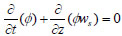
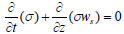
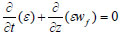
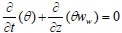
2.1. Development of the Three-Phase Model
The three-phase model was developed based on the following assumptions:
- Sand particles are spherical and of same size.
- Sand and oil or sand and water cannot mix.
- Oil is incompressible and the pipe is smooth.
- Effect of eddies is significant and deposit consists entirely of sand.
- Oil is Newtonian, sand particles mobility is as a result of the surrounding oil/water phase and the effect of forces including gravity, fluid-particle interaction and inertia forces.
Details on these assumptions and the developed model are presented in Appendices A and B, respectively.
 |
(1) |
 |
(2) |
 |
(3) |
 |
(4) |
 |
(5) |
 |
(6) |
 |
(7) |
3. THEORY CALCULATIONS AND MODEL SOLUTION
3.1. Determination of Model Constants/Calibration of Model
The new model, that is, the three-phase flow model was calibrated based on the explanations of Sanni et al. [13]. Finite difference solutions for the separate equations were then established with the different variables and lumped parameters estimated. The mass and momentum equations were solved based on upstream data shown in Table 1.
3.2. Boundary Conditions
Boundary conditions were established for each of the three components of the mixture
 |
(8) |
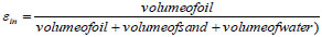
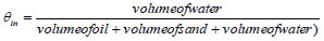
= 259.47/491.38 = 0.528 (oil concentration at the inlet)
 |
(9) |
= 177.376/491.38 = 0.361 (% water volume at inlet)
Then, φ,in = 1−(0.528+0.361) = 0.111 (sand concentration at pipe inlet) or 54.54/491.38 = 0.1110
Since
 |
(10) |
At the outlet,
 |
(11) |
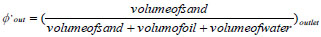
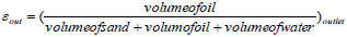
= 43.97/397.79 = 0.1105 is the sand concentration at pipe outlet and the corresponding ε and θ values (oil and water concentrations respectively) are:
 |
(12) |
= 210.02/397.79 = 0.528
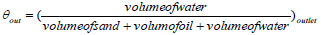 |
(13) |
= 142.99/397.79 = 0.359
3.3. Boundary Conditions for Sand, Water and Oil Momentum Equations
Equation 14 was used to estimate the concentrations knowing the boundary concentrations for the three components of the mixture.
 |
(14) |
Equal lengths at an interval of 6 m were marked out on the pipeline from 6-24 m. It was reasonable to also assume equal change in sand, oil and water concentrations since it is evident from the calculations that concentrations only varied slightly between the pipe inlet and exit for all three components: for sand 0.111, 0.110875, 0.11075, 0.110625, 0.1105 at t = 1 h from the pipe inlet through to its outlet respectively. For crude oil, the corresponding concentrations are: 0.52804347, 0.52802435, 0.52800523, 0.52798611, 0.5279670 while for water, the corresponding concentrations are 0.361, 0.360625, 0.36025, 0.359875, 0.3595. In order to further validate this claim, for a tubular or plug flow system, there is no variation in concentration with time at specific positions in the pipe as there is no back mixing and molecule history is not known as the molecules in the mix flow past spaces displacing other molecules.
The inlet velocities for the sand, oil and water (that is, 0.078 m/s, 0.371 m/s and 0.254 m/s respectively) were calculated based on the data along the first row in Table 1 and they were used as inlet boundary conditions for the momentum equations while 6.67 x 10⁻⁵ m/s, 6.67 x 10⁻⁵, 3.24 x 10⁻⁴ m/s and 2.2 x 10⁻⁴ m/s were estimated as their corresponding outlet velocities. The boundary conditions were established based on data with pressures between 793-1100 psia which gave the least amount of produced sand but highest amount of crude oil.
3.4. Solving the Mass Conservation Equations
3.4.1. Finite Difference Formulae for the Mass Conservation Equations
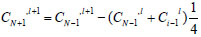
Equations 15-18 are the finite difference equations for the sand, water and oil phase mass conservation equations respectively.
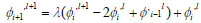 |
(15) |
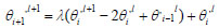 |
(16) |
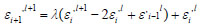 |
(17) |
 |
(18) |
The calculated λ = 5.66 x 10⁻⁴ and an average value for sand diffusivity was obtained from the values obtained at the inlet and outlet, that is, 1.132 x 10 -5 m2/s so as to simplify the simulation.
A solution was established for the mass conservation equations using Equations 15-18 where l represents position and i represents time e.g. 6 m away from pipe inlet, l+1 = 6 m and time t = 1 h.
Dt is the sum of molecular and eddy diffusivity terms.
By applying Equation 14 to the solid phase mass conservation equations, the last three points (that is, the 6 m, 12 m and 18 m points) are considered in calculating the exit (24 m) concentration.
φi,l+1 = 5.66*10−4 (0.110875−2(0.11075) + 0.110625) + 0.11075 = 0.11075
The calculated exit concentration for sand using the three phase model = 0.11075
while at the field, the sand concentration at the exit is 0.1105.
Hence, % difference/error =  and this implies the predicted sand concentration at the exit per hour is 99.77% accurate when compared to the result from the field considering 1 hour time step and a total time of 24 hours.
Similarly, for water, considering the 6 m, 12 m and 18 m sections of the pipe, the % volume of water, is given by Equation 16:
θi+1,l+1 = 1.93×10−3*(0.360625−2*0.36025 + 0.359875) + 0.359875 = 0.359875
The average total diffusivity between the inlet and outlet is 3.86 x 10⁻⁵ and from Equation 18, λ = 1.93 x 10⁻³.
At the field, % volume of water at the pipe exit = 0.3595 while the predicted volume % of water = 0.359875.
% error =  = 0.10% which is 99.9% accurate.
Applying Equation 17 to the oil phase mass conservation equation, for an average sum of eddy and molecular diffusivities of 5.8495 x 10⁻⁵, λ = 2.925 x 10⁻³
Considering the 6, 12 and 18 m sections of the pipe at t = 1 h implies,
εi+1,l+1 = 2.925×10−3*(0.528024−2*0.528005 + 0.527986) + 0.528005 = 0.528005
The actual exit oil concentration = 0.527967 and the predicted oil concentration is 0.528005
% error = 0.0072% which means the result is 99.99% accurate.
To estimate the corresponding amount of sand from the model, experimental results have to be considered. Based on measurements, 0.1105 sand concentration at the exit corresponds to 1.22 pptb then, 0.01075 from finite difference calculation gives:
 = 1.227 pptb which gives 99.5% accuracy.
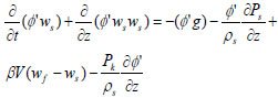
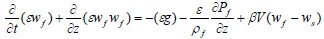
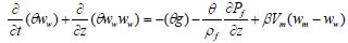
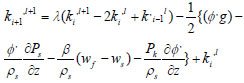
3.4.2. Finite Difference Formulae for the Momentum Conservation Equations
φ,ws, εwf θww were obtained by multiplying the volume fraction of sand, oil and water by their corresponding velocities, that is, 0.078 m/s, 0.371 m/s and 0.253 m/s are the inlet velocities obtained for sand, oil and water respectively while their corresponding outlet velocities are 6.67×10⁻⁵m/s, 3.2×10⁻⁴m/s and 2.2×10⁻⁴m/s.
 |
(19) |
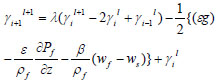 |
(20) |
 |
(21) |
Equations 19-21 are the momentum equations for the sand, oil and water phases respectively, where:
k = φ,ws, γ = εwf and Ω = θww.
3.5. Model Validation
In order to confirm the new three phase model’s accuracy, sand production data obtained from experiments were compared with the model estimates at the flow conditions; See (Table 2).
| Run (-) | Oil+water BLPD (bbl) | Amount Oil Exp. BOPD (bbl) | Amount Oil & Doan et al. [6] & Sanni et al. [13] models BOPD (bbl) | Amount Oil New model BOPD (bbl) | Produced sand exp. (pptb) (lb/mbbl) | Produced Sand Doan et al. [6] & Sanni et al. [13] (lb/mbbl) | Produced Sand new model (pptb) (lb/mbbl) |
|---|---|---|---|---|---|---|---|
| 1 | 2343 | 1237.0267 | 1237.0267 | 1237.03 | 1.31 | 0.30942 | 1.30699 |
| 2 | 1797 | 948.76 | 948.7567 | 948.757 | 1.31 | 0.30942 | 1.30699 |
| 3 | 2198 | 1160.47 | 1160.4715 | 1160.47 | 1.31 | 0.30942 | 1.30699 |
| 4 | 2293 | 1210.63 | 1210.6283 | 1210.63 | 2.55 | 0.60231 | 2.54414 |
| 5 | 2375 | 1253.92 | 1253.9216 | 1253.92 | 2.55 | 0.60231 | 2.54414 |
| 6 | 2311 | 1109 | 1106.4493 | 1106.45 | 2.65 | 0.62593 | 2.63675 |
| 7 | 2467 | 1204 | 1201.2308 | 1201.23 | 2.65 | 0.62593 | 2.63675 |
| 8 | 2498.1 | 1202 | 1199.2345 | 1199.23 | 2.88 | 0.680256 | 2.8656 |
| 9 | 2503.3 | 1194 | 1191.2538 | 1191.25 | 2.88 | 0.680256 | 2.8656 |
| 10 | 1729 | 761 | 759.2497 | 759.24 | 3.01 | 0.710962 | 2.99495 |
Table 2 gives the results obtained for sand production data from experiments as compared with those calculated using the Sanni et al. [13] two phase model and the new model (that is, the three-layer/phase model) discussed in this work that considers the water phase alongside sand and crude oil.
(i) Evaluation of solid phase pressure forces
The solid and fluid phase pressures were determined by simply estimating the product of ϕ’*ps and ε*pf rather than applying Equation 21 also known as the single phase Sthumiller [15] pressure model as suggested in Sanni et al. [13]. The conceptual deviation is more reasonable because, the whole stream flows as a mixture of phases thus, the phases will only separate out based on the flow conditions and particularly the Reynolds, Euler and Froude numbers which are force ratios of inertia to viscous forces, pressure to inertia and inertia to gravity forces respectively.
 |
(22) |
Note:
The phase pressures are actually products of the volume fractions of the components of the mixture.
(ii) Evaluation of kinematic forces for solid phase momentum equation
The kinematic pressure equation as given in [6] is given by Equation 23.
 |
(23) |
Since sand concentration is less than 20% throughout the pipe cross-section, it then implies that Equation 24 for dilute suspension applies [6].
 |
(24) |
Hence, h(0.111) = 1.596
:. the corresponding 
When t = 1 hour, at the inlet, there is no gradient in sand concentration, so the gradient multiplier makes the function undefined thus, the product of Pk/ρs and concentration gradient values can be calculated at other points ; since Δz can be evaluated 6 m away from pipe inlet, where (ϕ) = 0.11087 and t = 1 hour, there would be need to do some evaluation to get the corresponding h (ϕ)
Hence, h (0.110875) = 1.5959 and Pk = 65.47 kg/ms2
12m away, where, (ϕ) = 0.1107, by calculation, h (ϕ) = 1.5950 and Pk = 29.12 kg/ms2
18m away, where, (ϕ) = 0.11062 and by calculation, h (ϕ) = 1.594 and Pk = 7.3 kg/ms2
At the exit, (ϕ) = 0.1105, h (0.1105) = 1.5932 and Pk = 0.000087 kg/ms2
The same procedure applies at other times along the pipe length considering a time step of one hour and a total time of 24 h.
(iii) Evaluation of ϕg
Taking g = 9.81 m/s2, when t = 1 hour, at the pipe inlet, then
 = 0.5 x 0.111 x 9.81 = 0.545 m/s2
6m away from pipe inlet, (ϕ) = 0.11087 then,
 . The same procedure applies at other points for t = 1 hour and at further times along pipe length considering a time interval of 1 hour and a time total of 24 hours.
(v) Evaluation of εg
When t = 1 h, at the pipe inlet, ε = 0.945 then,  and 6m away, ε = 0.52802435 then,
  and so on, as explained for the solid phase.
(v) Evaluation of θg for the water phase,
At t = 1 h, at the pipe inlet, θ = 0.361 then, 
6m away, θ = 0.360625 then,  and so on, as explained for sand and crude oil phases.
(vi) Evaluation of 
The interaction coefficients along the axial distance were determined using (25).
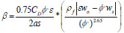 |
(25) |
The reason is because, ϕ < 0.20 (dilute suspension)
To evaluate β, there is need to calculate, s, s+ and CD
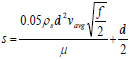 |
(26) |
and
 |
(27) |
Givler and Mikatarian [7] gave expressions for estimating the friction factor of a particle in a flowing fluid for laminar flow where Re≤1000,
 |
(28) |
For transitional flow, Re > 1000 < 2100 while for turbulent flow Re is greater than 2100 although, some literature say turbulence begins at Re > 4000 based on pipe diameter.
 |
(29) |
But,
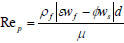 |
(30) |
where Rep = particle Reynolds number, ρf fluid density, f = friction factor, d = pipe diameter, ε = fluid concentration, ϕ = solid concentration, μ = fluid dynamic viscosity, wf, ws = fluid and solid velocities respectively.
The dimensionless stopping distance of a particle is a measure of the ratio of: the product of the particle’s stopping distance (distance of travel before it meets an obstacle), its friction factor and particle velocity to, the kinematic viscosity of particle, that is, the ratio of particle resistance to the fluid’s kinematic viscosity. When particle Reynolds number, Rep < 1000,
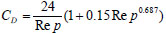 |
(31) |
but,
CD = 0.44 when Rep > 1000
where:
CD = drag coefficient
However, for 0.111 sand concentration at the inlet, ws = 0.078 m/s and, wo = 0.371 m/s.
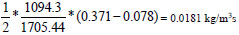
At z = 0 m, using Equation 25, β = 1094.3 kg/m3s.
Therefore, at the inlet, where t = 1 h
 implies,
6 m away, β = 282.05 kg/m3s then,
 gives:
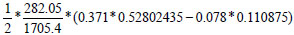 = 0.094 m2/s and so on.
For the crude oil and water, the same procedure applies at all points down to the exit for the entire time.
3.6. Force Ratio Analyses
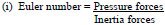
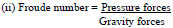
A force ratio relationship was performed in order to know the contribution of each of the forces already mentioned in section 1.0 to the transport process. The combined mechanisms of interest include Euler, Froude, Reynolds and Schmidt numbers. Table 3 shows the mechanisms of interest and the variables they consist.
| Item | Mechanisms | Variables/Model Parameters |
|---|---|---|
| A | Inertia forces |
 (velocity and diameter) (velocity and diameter) 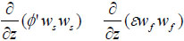
|
| B | Pressure forces |
 or Re/mix viscosity or Re/mix viscosity  (pressure, density and diameter) (pressure, density and diameter) 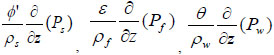
|
| C | Viscous forces |
 (kinematic viscosity, velocity and diameter) Re/inertia forces (kinematic viscosity, velocity and diameter) Re/inertia forces |
| D | Gravitational forces | ϕ'g, εg, and θg |
| E | Momentum and molecular diffusivities | η and D (kinematic viscosity and diffusion coefficient) |
The values for the force ratios are estimated thus:
At 0 metre, the pressure forces are undefined. In essence, no value was estimated at 0 metre at all times. When t = 1 h:
 |
(32) |
 |
(33) |
 |
(34) |
(iv) Schmidt number = Momentum diffusivity
Molecular diffusivity
 |
(35) |
From the calculations, the estimated effective diffusivity De = 0.0000132 m2/s at the pipe exit.
Note:
The sum of molecular and eddy diffusivity = total diffusivity and  = 0.342 is the average value of the Schmidt number. Considering the molecular and momentum diffusivity values for the sand particles. This ratio being so small implies that, the molecular diffusivity is higher relative to momentum diffusivity for the particles. The average value of the Schmidt number for a spherical particle is 0.9 from literature. This value may be accurate for fines since they are smaller and diffuse faster but in this work, medium sand size particles were considered. Also, there could be some variations that, is, in fluid rheology such as density and viscosity along with particle size, etc. in the three regions (sub-laminar, transition and turbulent cores) considered whereas, the Fick’s Equation for diffusion that was used to estimate the molecular diffusivity does not incorporate these changes although, the effect for eddies were accounted for. The aforementioned dimensionless numbers were obtained after solving the momentum equations. The results for the force competitions can be seen in Tables (4, 5 and 6). Schmidt number was determined and assumed constant throughout the transport process.
| t (hrs) | 0 m | 6m | 12 m | 18 m | 24 m |
|---|---|---|---|---|---|
| 1 | 0.01631 | 0.02174 | 0.03259 | 0.065058838 | 18.9646 |
| 2 | 0.01631 | 0.02174 | 0.03259 | 0.065058838 | 18.9646 |
| 3 | 0.01631 | 0.02174 | 0.03259 | 0.065058838 | 18.9646 |
| 4 | 0.01631 | 0.02174 | 0.03259 | 0.065058838 | 18.9646 |
| t (hrs) | 0 m | 6m | 12 m | 18 m | 24 m |
|---|---|---|---|---|---|
| 1 | 0.00974 | 0.01298 | 0.019461029 | 0.03885 | 11.2183 |
| 2 | 0.00974 | 0.01298 | 0.019461029 | 0.03885 | 11.2183 |
| 3 | 0.00974 | 0.01298 | 0.019461029 | 0.03885 | 11.2183 |
| 4 | 0.00974 | 0.01298 | 0.019461029 | 0.03885 | 11.2183 |
| t (hrs) | 0 m | 6m | 12 m | 18 m | 24 m |
|---|---|---|---|---|---|
| 1 | 0.00666 | 0.00888408 | 0.0133184 | 0.026591 | 7.71258946 |
| 2 | 0.00666 | 0.00888408 | 0.0133184 | 0.026591 | 7.71258946 |
| 3 | 0.00666 | 0.00888408 | 0.0133184 | 0.026591 | 7.71258946 |
| 4 | 0.00666 | 0.00888408 | 0.0133184 | 0.026591 | 7.71258946 |
4. RESULTS AND DISCUSSIONS
The produced sand and crude oil obtained from experiments were compared with estimates of sand and crude oil from Doan et al. [6], Sanni et al. [13] models and the new three-phase model. In Table 2, for a total of 10 runs, the quantity of produced oil calculated by the Doan et al. [6], Sanni et al. [13] models and the new three phase model compared favourably with the values obtained from experimental data with the models giving high levels of accuracy (that is, over 99 % accuracy). However, for the produced sand in pounds per thousand barrel, the Doan et al. [6] and Sanni et al. [13] gave poor estimates with error of 76.38 % while the new model gave better predictions with high precision of over 99.77 % or 0.23 % error. The reason for the poor performance of the Doan et al. [6] and the Sanni et al. [13] models relative to the newly developed model is the amount of associated water accompanying the sand phase. Based on the analyses, it was discovered that for low water cut reservoirs, the amount of water is low hence the Sanni et al. [13] model is less prone to errors when used for sand estimation. As the water cut in the reservoir fluid tends to zero, the new model reduces to the Sanni et al. [13] model. However, for very low water cut reservoirs, the Doan et al. [6] and the Sanni et al. [13] can give good estimates of the amount of oil recovered from the well but become more prone to errors as the quantity of associated water in the oil increases (Fig. 1).
4.1. Effect of Reynolds Number
Reynolds number helps to characterize a flow system and also gives insight to the ratio of the magnitude of inertia to viscous forces at the flow conditions. From the calculated Reynolds numbers for sand, it is evident that almost all the sand particles were in the turbulent region between the 0 and 6 m points. The region characterized by the flow at the 0 – 12 m point, shows that the sand particles were between the turbulent core and the transition zone while beyond the 18 m point, the particles were already in the laminar regime. Reynolds number at or below 1000 reveals that flow is laminar, Re >1000 but less than 2300 reveals that the flow is in the transition zone and Re > 2300 shows that the flow is turbulent.
In the contour plot of Fig. (2), the Reynolds number of the sand phase for the first four hours varied between 3924.8 and 3.4 from the inlet down to the exit respectively although, the value at each point was constant between 1 and 4 hours. This region lies between the dark blue (laminar region) and red (laminar, laminar sub-layer, transition zone and turbulent region) regions which are close to the pipe wall. It dropped significantly at the inlet probably because of the type of screen (coarse screen) the mixture was in contact with between the 0 and 6 m points. Coarse screens help to sieve out of the mixture, the largest of sand particles which are also capable of forming a sand cake around and on the screen surface over time thus reducing the influx velocity, flow rate and pressure. Different screen sizes are integrated within upstream petroleum pipelines ranging from very coarse to coarse, medium, fine and very fine screens based on their mesh sizes and sand information obtained from the production/formation zone. However, from the estimated Reynolds numbers obtained at the 6, 12, 18 and 24 m points, that is, 3924.8, 2944.4, 1964.1 and 3.4. It is obvious that subsequent screens could also be responsible for flow reductions which then resulted in increased pressure drop hence, the flow conditions were altered since the change in Reynolds number from point to point shows that, the 12 to 24 m points should be given special attention in order to avoid cases of flow seizure. Between the 12 and 18 m points, a moving bed of sand may be formed, however, its continuous movement will cause stress corrosion cracking of the pipe as the sand grains may grind off some metallic grains of the pipe along the pipe’s grain boundaries. For the 18 m and 24 m segment of the pipe, a stationary bed may result which in turn reduces the flow area and imparts some momentum on the oil thus causing oil to flow with a higher velocity through the available space above the sand bed. This goes further to imply that, at some critical conditions, oil recovery may still be evident owing to the influence of the moving bed on the oil however, here, the bed height of the sand particles becomes significant.
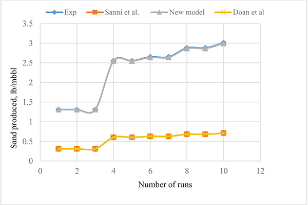 |
Fig. (1). Profile of experimental and model estimates of produced sand at the well head. |
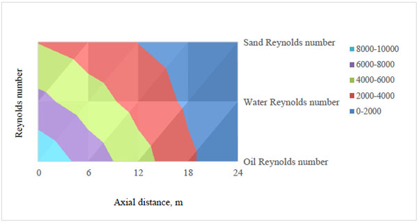 |
Fig. (2). Reynolds number of sand, oil and water at different times along the axial distance. |
As discussed for the sand phase, between 1 and 4 hours, the Reynolds number of the oil phase was 9602 at the pipe inlet and lowest (8) at the exit; this region lies between the dark blue laminar layer to the light blue turbulent core region. Here, the change is most significant between the 18 and 24 m points based on the underscored reason for the sand phase in terms of pressure drop, screens and sand deposit formation within the line between those points. At the 6, 12, 18 and 24 m points, the calculated Re are 7204, 4805, 2406 and 8 respectively for the first four hours. Although high Reynolds numbers are desired, the values at the inlet and 6 m points should also be checked because high turbulence begins at or above 4000 and if the flow rate is far too high, it can result in pipe hammering or knocking which could impart unbearable pressures on the pipe walls thus resulting in pipe burst/rupture. Despite the degree of turbulence desired, it should be moderated such that the Re is about half this value, so that with the help of boosters/pumps it becomes safe to transport the entrained sand and water. Considering all points from the inlet down the exit, since Re is the ratio of inertia to viscous forces, one can infer from the estimated Reynolds numbers that inertia forces (ensuing from the flow velocities) dominate the viscous forces which tend to oppose the movement of the reservoir fluid; the inertia forces at the exit still show that the inertia forces are 8 times the magnitude of the viscous forces hence, it is reasonable to still have oil recovered based on the magnitude of the oil pressure at the pipe exit. Furthermore, despite the desire to have high inertia forces, it is also reasonable to consider equipment/pipe integrity at any flow condition. The inertia forces surpass the viscous forces to a good measure at the 0 and 6 m points which raises concern for pipe safety while at the outlet, operations in the industry, gave reports on pressure drop and flow anomalies that were regulated to prevent plugging and pigging operations. Furthermore, it is recommended that the Re be maintained far above the condition for critical flow for enhanced oil recovery.
For the water, the estimated Reynolds number was seen to decrease from the inlet to the exit between 1 and 4 h. It was approximately 66572, 4930, 3289, 1647 and 6 at the 0, 6, 12, 18 and 24 m points respectively; this region is characterized by the dark blue laminar layer to the purple turbulent core region. Although, it is good to keep the Re high enough so as to keep the water phase suspended in the flowing stream because at critical conditions, the Re being too low will cause water and deposited sand to rest on the pipe wall which is unsafe for the pipe as corrosion and pipe abrasion may set in from bed load transport of the sand, that is, if the deposited sand forms a moving bed at the flow conditions. If a stationary bed results, it then means partial or total plugging of the pipe may result which will either confine the flow to a region above the deposit or completely restrict flow as the case may be.
Tables 4-6 give the calculated friction factors for the sand, water and oil phases respectively. The friction factors seem to rise from the pipe inlet to the exit for all three components although, the friction factor of the sand is highest while that of the oil phase is least with that of the water phase being higher. It is evident that the densities and phase velocities of the different components have significant influence on their friction factors. Furthermore, the drop in flow rates of the carrier fluid, sand and water is also responsible for the reduction in Reynolds numbers for all components of the mixture from the pipe inlet through to the exit. Fig. (3) is a plot of the variation of the friction factors of the three components within the first four hours and along the axial distance. The plot shows that the friction factor increases along the axial distance and is highest for the sand phase, that of water is next in magnitude while the oil phase has the least friction factor.
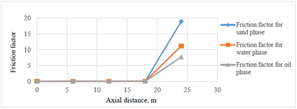 |
Fig. (3). Friction factor for sand, oil and water along the axial distance. |
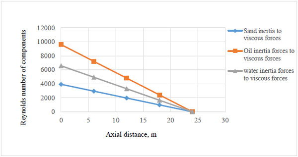 |
Fig. (4). Reynolds number of components along the axial distance. |
The Reynolds numbers of the components as shown in Fig. (4). decrease along the axial distance. This is as a result of the reduced velocities. As the velocities of the components decreased from the pipe inlet to the exit, corresponding reductions can also be seen for the three components. However, oil being the lightest of the three components showed the least reduction in Reynolds number while that of water was higher with sand having the lowest Reynolds numbers along the pipe axis.
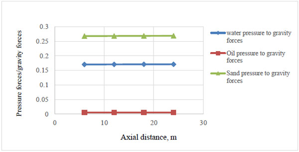 |
Fig. (5). Ratio of pressure to gravity forces for oil, sand and water along the axial distance. |
For the first four hours, the ratio of pressure to gravity forces as shown in Fig. (5) in decreasing order of magnitude for the components is sand, water and oil. This is simply due to the fact that these forces are measures of the concentrations of the three components, that is, it is as a result of the difference in concentration of sand, oil and water from point to point along the pipe axis.
 |
Fig. (6). Froude number of oil, sand and water along the axial distance. |
Fig. (6) gives an illustration of the force competition between inertia and gravity forces. Inertia forces of the three components of the mixture are functions of their velocities while their gravity forces are measures of the concentration distribution of the three components in the mixture that is, where velocity is highest, inertia force is maximized and where concentration is highest, gravity force is maximized and vice-versa. The Froude number of oil is highest, next to it is that of water and that of sand is lowest between 0-4 h of well production time. This goes further to imply that, considering Figs. (5 and 6), in order to operate and maintain the pipe within reliable and safe flow conditions, it is necessary to keep the inertia forces high by integrating a booster at some point mid-way between the pipe terminals. This is so as to make up for the lost inertia forces thus controlling/reducing the sand phase pressures exerted by the agglomeration of sand or clustering sand or water molecules at critical points within the flow system. Because, towards the exit, the drop in inertia forces tend towards the critical deposit velocity thus increasing the frictional forces in the pipeline.
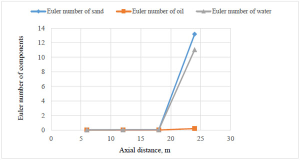 |
Fig. (7). Ratio of pressure to inertia forces for oil, sand and water along the axial distance. |
In Fig. (7), The force competition between the pressure and inertia forces shows that the critical point for controlling phase pressures is the 12-18 m points beyond which pressure forces begin to dominate the inertia forces of sand and water which must not settle on the pipe wall if the pipe integrity must be maintained/sustained.
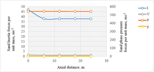 |
Fig. (8). Force distribution of the sand particles across the pipe. |
For further investigation, the model was tuned in order to see the effect of the underscored mechanisms as the flow becomes stratified at lower Reynolds number. Fig. (8) confirms the need to step up the inertia forces (I) against the gravity forces (g) and pressure forces (P) at Reynolds number of 300 where the flow is laminar, that is, higher Euler and lower Froude numbers are required to keep the stream flowing as a continuum or suspension as this will also help to reduce the tendency of having water and sand confined to the pipe wall. Also, under this condition, the value of sand gravitational or sand pressure forces are higher than the inertia or viscous forces (V) of the carrier crude oil.
Using the Stuhmiller model [15], the interfacial pressures of the components were determined. The sand, crude oil and water densities used are 1705.4, 878 and 1000 kg/m3 respectively. At the surface of a sphere, the normal force exerted at the surface is at 90o to the surface. The estimated interfacial pressures on hourly basis show that the interfacial pressure at the oil-water interface is higher than the interfacial pressure at the water-sand interface and the pressure between the sand phase and the pipe wall which are in the range of 815352.6-811797.6 kgm-1-s2, 3866799-4003121 kgm-1-s2 and 2444847-2725780 kgm-1-s2 respectively. This is due to their respective densities and flowing velocities under the flow conditions see Fig. (9). The ease with which oil will rub or slide over water is higher than the rate of flow of water over the sand phase and from the estimated pressures, it shows that as the flow conditions become critical, the sand and water interaction may become detrimental to the pipe. However, efforts should be made to keep the stream flowing at pressures high enough to enhance oil-sand interaction by taking advantage of the repulsive force between oil and water since they do not mix thus, lowering the oil-water interaction force because, from the estimated interfacial forces, it is somewhat evident that the oil-sand interaction force may get worse towards the pipe exit.
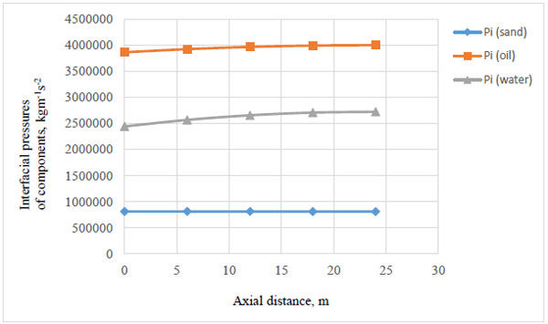 |
Fig. (9). Interfacial pressure of the components along the axial distance. |
CONCLUSION
The results from the simulation show that the model gives good description of the forces responsible for the flow of a mixture of sand, crude oil and water through horizontal pipes in oil wells. From the calculated forces, one could see at a glance that Euler number seemed to show significant variations beyond the 18 m point where the pipe integrity may be at stake depending on the nature of the flow regime and drag force on the pipe walls. The Froude number of the three components showed significant variations from the inlet to the exit of the pipe and as stated earlier, the critical points for consideration during monitoring operations should be the 12-18 m points beyond which the pressure forces begin to compete favourably with/dominate the inertia forces. Furthermore, in order to prevent sand deposition in a petroleum pipeline, the inertia forces imparted by the carrier oil must essentially dominate the sand phase pressure and gravity forces.
NOMENCLATURE
| Symbols | Designation | Unit |
|---|---|---|
| Letters | ||
| A | Cross-sectional area | m2 |
| g | Gravitational acceleration | ms-2 |
| Pf | Oil phase pressure | kgm-1s-2 |
| Pk | Kinematic pressure | kgm-1s-2 |
| Ps | Sand phase pressure | kgm-1s-2 |
| Pw | Water phase pressure | kgm-1s-2 |
| qf | Volume flow rate of oil | m3s-1 |
| qs | Volume flow rate of sand | m3s-1 |
| qw | Volume flow rate of water | m3s-1 |
| t | Time | hrs or s |
| Vm | Volume of mixture | m3 |
| wo | Oil velocity | ms-1 |
| ws | Sand velocity | ms-1 |
| ww | Water velocity | ms-1 |
| z | Axial distance | m |
| β | Fluid-particle interaction coefficient | kgm3s-1 |
| Δz | Change in length | m |
| ε | Oil concentration (volume fraction) | - |
| ϕ | Suspended sand concentration (volume fraction) | - |
| σ | Deposited sand concentration (volume fraction) | - |
| ϕ’ | Total sand concentration (volume fraction) | - |
| θ | Water concentration (volume fraction) | - |
| ρf | Oil density | kg/m3 |
| ρs | Sand density | kg/m3 |
| ρw | Water density | kg/m3 |
LIST OF ABBREVIATIONS
| BLPD | = Barrels of liquid per daybbl/day |
| BOPD | = Barrels of oil per day bbl/day |
| BSW | = Base sediment & water % |
| Choke | = Choke size - |
| FTP | = Flowing tubing pressure Psia |
| Gas | = Amount of gas produced scf/d |
| GOR | = Gas oil ratio - |
| GL rate | = Gas-liquid rate scf/day |
| Pinj | = Injection pressure Psia |
| PTB | = Parts per thousand barrel pptb |
CONSENT FOR PUBLICATION
Not applicable.
CONFLICT OF INTEREST
The authors hereby declare that there is no conflict of interest of any sort as regards the publication of this article as all contributors have been included with the sponsors duly acknowledged.
ACKNOWLEDGEMENTS
The authors wish to thank ADDAX oil Limited and Department of Petroleum Resources Nigeria Ltd for their contributions in making this research work a success. Also, Covenant University is appreciated for her sponsorship and support in liaison with the company management at a time it was necessary and while the work was in progress. The authors also appreciate Samuel Sanni for carrying out the research and preparing the manuscript, Samuel Adefila for his contributions and useful suggestions, Ambrose Anozie for his contributions, revision and involvement in the mathematical simulations and Oluranti Agboola for revising and editing the manuscript.
REFERENCES
| [1] | Adeyanju OA, Oyekunle LO. Hydrodynamics of oil-sand-gas multiphase flow in a near vertical well Nigerian Annual Conference and Exhibition 2012; 1-17.6-8 August; Abuja, Nigeria. 2012; pp. |
| [2] | Berrone S, Marro M. Space-Time Adaptive Simulations for Unsteady Navier Stokes Problems 2009; 38: 1132-44. |
| [3] | Boulanger JA, Wong CY. Sand suspension deposition in horizontal low-concentration pipe flows. Granul Matter 2016; 18(2): 1-10. |
| [4] | Chu KW, Kuang SB, Yu AB, Vince A. Particle scale modelling of the multiphase flow in a dense medium cyclone: Effect of fluctuations of solid flow rate 2012; 33: 34-45. |
| [5] | Davarzani H, Marcoux M, Costeseque P, Quintard M. Experimental measurement of the effective diffusion and thermodiffusion coefficients of binary gas mixture in porous media. Chem Eng Sci 2010; 65(18): 5092-104. |
| [6] | Doan Q, Farouq A, George A, Oguztoreli M. Sand deposition inside a horizontal well - A simulation approach. SPE J 2000; 39: 33-40. |
| [7] | Givler RC, Mikataranian RR. Numerical simulation of fluid-particle flows: Geothermal drilling applications. J Fluids Eng 1987; 109(3): 324-31. |
| [8] | Horender S, Hardalupas Y. Fluid-Particle Correlated Motion and Turbulent Energy Transfer in a Two-Dimensional Particle-laden Flow 2010; 65: 5075-91. |
| [9] | Jia H, Dang R. Development of contactless sand Production Instrument. Open Petroleum Engineering Journal 2016; 10: 1-11. |
| [10] | Kawano S, Sei A, Kunitake M. Thixotropic Interparticle Interaction between Silica and non-Ionic Polymer Particles Prepared by Static Dispersion Polymerization. Polymer (Guildf) 2011; 52(7): 1577-88. |
| [11] | Liu Y, Liu X, Li G. Numerical Investigation on Hydrodynamics of Gas Binary Particles Flows Using a Second-Order-Moment Turbulent Model 2012; 72: 58-107. |
| [12] | Rahmati H, Jafarpour M, Azadbakht S, et al. Review of Sand Production Prediction Models. Journal of Petroleum Engineering 2013; 2013: 1-16. |
| [13] | Sanni SE, Olawale AS, Adefila SS. Modeling of sand and crude oil flow in horizontal pipes during crude oil transportation. J Eng 2015; 2015: 1-7. |
| [14] | Sanni SE. 2016. “Modelling of Sand Entrainment and Deposits in Horizontal Oil Transport” A.S. Olawale, & S.S. Adefila Eds., Deutschland, Germany: Verlag, Scholar’s Press, 2016, pp. 60-100. |
| [15] | Stuhmiller JH. The Influence of Interfacial Pressure Forces on the Character of Two Phase Flow Model Equations. Int J Multiph Flow 1977; 3: 551-60. |
| [16] | Wang B. Interface interaction in a turbulent vertical channel flow laden with heavy particles. part I: Numerical methods and particle dispersion properties. Int J Heat Mass Transfer 2010; 53: 2506-21. |
| [17] | Zhou SZ, Zhang S, Lv ZP, Qin L. Research and simulation of solids-conveyance law of the shale shaker. Open Pet Eng J 2016; 9 |
| [18] | https://en.wikipedia.org/wiki/Mechatronics Received 2 March, accessed |