
RESEARCH ARTICLE
Lattice Boltzmann Simulation of Natural Convection in a Fractured Petroleum Reservoir Domain: Single-Phase and Multi-Phases Investigations
Hossein Kaydani1, Ali Mohebbi1, *, Amir Ahmad Forghani2
Article Information

Identifiers and Pagination:
Year: 2018Volume: 11
First Page: 48
Last Page: 66
Publisher Id: TOPEJ-11-48
DOI: 10.2174/1874834101811010048
Article History:
Received Date: 23/2/2018Revision Received Date: 4/04/2018
Acceptance Date: 12/04/2018
Electronic publication date: 30/4/2018
Collection year: 2018
open-access license: This is an open access article distributed under the terms of the Creative Commons Attribution 4.0 International Public License (CC-BY 4.0), a copy of which is available at: https://creativecommons.org/licenses/by/4.0/legalcode. This license permits unrestricted use, distribution, and reproduction in any medium, provided the original author and source are credited.
Abstract
Background:
Natural convection is one of the main effective production mechanisms in a fractured petroleum reservoir.
Objective:
This paper investigated the simulation of natural convection heat transfer in a fracture domain of petroleum reservoir.
Methods:
This is done by using Lattice-Boltzmann Equation (LBE) method. In this study, a D2Q9 lattice model was coupled with the passive-scalar lattice thermal model to represent density, velocity and internal energy distribution function, respectively.
Results and Conclusion:
The results were in excellent agreement with CFD results from the literature. The effects of Rayleigh number and Aspect-Ratio (AR) on flow pattern and temperature distribution were studied. The results indicated that natural convection rate increased with the Rayleigh number increment. The local Nusselt number (Nu) was evaluated on the hot wall and it was rising with increasing the Rayleigh number. Streamlines and temperature field were affected significantly by changing the aspect-ratio. Moreover, first of all, natural convection in Single Component Mutli-Phase (SCMP) was discussed and here and then after validation of SCMP model, the results indicated that the streamline and isotherm were affected by second phases because of the formation of two-phase flow in some of the reservoirs or production period.
1. INTRODUCTION
Natural convection is a very common phenomenon in several engineering and environmental problems, where the motion drives by the interaction of a difference in density with a gravitational field [1]. A large percentage of the world’s oil and natural gas is contained in fractured rocks of carbonate reservoir. Although the resources are extensive, the recovery of fluids from these reservoirs is hampered by our inability to excellently predict the production mechanisms of the fractures in these reservoir rocks. Natural convection in the fractured reservoir is one of the most effective mechanisms [2].
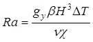
The conditions for the onset of convection can be determined by the value of the Rayleigh number (Ra), which is a dimensionless group that relates buoyant destabilizing forces to viscous and conductive restoring ones. The value of this parameter must exceed a certain critical value (Rac) to start the natural convection. For a layer of fluid enclosed between horizontal impermeable surfaces with a linear temperature profile, this value is well established as Equation 1 [3]:
 |
(eq 1) |
Many investigators studied flow and thermal distribution because of the natural convection in different problems [4-8]. Convection in porous media has been studied extensively over the last decades and can be categorized in theoretical and numerical studies. In theoretical studies, the onset of convection for different boundary and initial conditions was studied by using appropriate governing equations [2, 9-11]. However, some assumptions and simplifications were assumed to solve problems. Medina et al. [12] studied theoretically and experimentally the thermal convection in long tilted fractures filled with a porous material (porous layer) embedded in an impermeable solid and saturated with a fluid
They presented analytical expressions in low Rayleigh number flows for the temperature and velocity profiles in a porous layer model.
Numerical investigations of natural convection in gas, oil and water reservoirs were conducted by several studies. They reviewed different numerical approaches for better understanding of some quantitative aspects of natural convection in porous media [13-15]. Wang et al. [16] studied the onset of natural convection numerically in a finite, thin and vertical oriented saturated porous slab between two impermeable conducting blocks. Their results indicated that the presence of two contiguous conducting blocks changes the stability properties in the porous slab dramatically, because of the thermal interactions in the composite system. Moreover, the natural convection caused the composition variation in a column of reservoir fluid, which was studied numerically by some investigations [17, 18].
However, a few studies are available on natural convection in fractured zones, although this is a major mechanism for heat and mass transfer in carbonate rocks [19]. Moreover, the many aspects of this phenomenon and the most effective parameters that can affect the natural convection in a fractured petroleum reservoir need to be further investigated. The effects of fracture geometry and dimensionless parameters of heat transfer on the velocity and temperature profiles in natural convection for a fractured reservoir should be studied in details. The Lattice-Boltzmann Equation (LBE) method is a Computational Fluid Dynamics (CFD) technique, which has been developed as a new tool for simulating the fluid flow, heat transfer and other complicated physical phenomena [8, 20-24] LBE model is different from the traditional numerical methods, which solve the discrete macroscopic Navier-Stokes (N-S) or energy equations. The LBE is a micro and meso scale modeling method based on the particle kinematics and corresponding relations between the actual simulated statistical dynamics at a microscopic level and the transport equation at the macroscopic equation. It has many advantages, such as simple coding, easy implementation of boundary conditions and fully parallelism [25].
Despite the widespread studies carried out on the topic of single phase thermal free convection in cavities, the authors believe that multiphase aspects of the problem and specifically LBM implementation of the Single Component Multi-phase model (SCMP) is still worth considering. On the other hand, variation of the physical aspects of the problem, including Rayleigh and aspect ratio effects are also interesting at a geothermal point of view. Accordingly, the aim of this study is to propose numerical LBE solutions related to transient natural convection in a fractured zone of a petroleum reservoir, which is heated from below. In order to validate the simulations, the results are compared with the previous studies [26]. The effects of the Rayleigh number and aspect-ratio on flow pattern and temperature distribution is to be presented. Moreover, since a reservoir liquid phase may form gas phase during depletion and the reservoir fluid may exist as two phases in some operation conditions, a multiphase analysis of the system is also carried out.
2. LATTICE BOLTZMANN MODEL
2.1. Lattice Boltzmann Equation
The standard LBE with the Bhatnagar-Gross-Krook (BGK) estimation can be presented as below Equation 2 [27]:
 |
(2) |
In Equation 2, x shows the position in space, t is time, δt is the time step, fα is the particle distribution function (PDF) along the direction of αth, fαeq is its corresponding equilibrium PDF, eα is the particle velocity in the direction of αth, τ is the single relaxation time and finally N represents the number of discrete particle velocities.
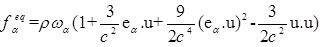
For 2-D flow, the nine-velocity LBE model on the 2-D square lattice can be applied which is, represented as the D2Q9 model. This model has been widely used in the literature. The equilibrium distribution for the D2Q9 model can be identified as below Equation 3 [27]:
 |
(3) |
In Equation 3, ω represents the weighting factor, c=δx/δt is the lattice speed, δx is the lattice step and u shows the macroscopic velocity.
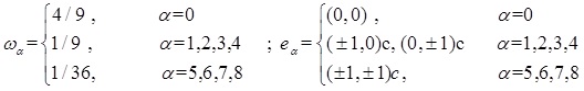
Below correlations are the weighting factor and discrete velocity for the D2Q9 model shown in Equation 4 [27]:
 |
(4) |
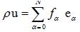
In most LBE simulations, Equation (2) can be solved with two steps. The first step is collision and the second step is streaming. In the collision step, the PDFs for each direction are relaxed toward quasi-equilibrium distributions then the distributions move to the neighboring nodes at the streaming step. The local mass density ρ and the local momentum density ρu are shown as below Equations (5, 6) [27]:
 |
(5) |
 |
(6) |
The Navier-Stokes (N-S) equations are recovered with LBE model for fluid flow near the incompressible limit and then the viscosity in the N-S equations is obtained as below [27]:
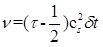 |
(7) |
In Equation 7, cs shows the lattice sound speed. So applying Equation 7 makes the LBGK scheme a second-order method to solve the incompressible flow [28].
2.2. Thermal Passive-Scalar LBE Model
In spite of the reasonable achievements on isothermal flow simulations, the thermal flow simulations have a great potential to be investigated. Generally, the existing thermal LBE models consist of two main categories such as the multispeed and the multi-distribution function approaches. The multispeed approach considers energy conservation by adding the higher-velocity terms in the equilibrium distribution but from theoretical aspect, the multispeed approach is instable numerically [29, 30]. The viscous heat dissipation and compression work with the pressure are considered negligible in the multi-distribution function approach so the temperature field is passively advocated with the fluid flow and then it can be solved with considering an independent temperature distribution function. This term is also called the passive-scalar approach which has better numerical stability and accuracy [31].
Energy equation can be solved in the LBE model framework. In this study, the D2Q9 model has been chosen as the velocity field. Consequently, the discrete Boltzmann equation for temperature field can be updated in Equation 8 [32]:
 |
(8) |
where τT shows the dimensionless relaxation time of temperature, gα is the temperature distribution function and finally, gαeq is the temperature distribution function at the equilibrium state and it can be calculated with below correlation in Equation (9):
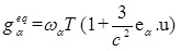 |
(9) |
where u represents whole fluid velocity. The temperature of the whole fluid T is considered with below formula in Equation 10:
 |
(10) |
In thermal model, the thermal diffusivity (X) is the key parameter in the simulation of a flow with heat transfer term and it can be expressed as below Equation 11 [32]:
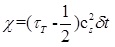 |
(11) |
The Prandtl number (Pr) for component, which related the kinematic viscosity (υ) and the thermal diffusivity (X) can be expressed as below in Equation 12 [32]:
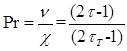 |
(12) |
2.3. Multi-Phase LBE Model
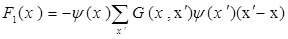
Microscopically, the reason for fluid system segregation into different phases is related to the inter-particle forces. In the single component multi-phase (SCMP), LBE model has been proposed by Shan and Chen. LBE model is a simple interaction potential model which is defined to describe the fluid/fluid interaction. Then the model incorporates the forcing with shifting the velocity in the equilibrium distribution. The fluid/fluid interaction force is defined as below Equation 13 [31]:
 |
(13) |
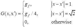
where x and x'(=x + eiδt) show the position in space G(x, x') and denotes intermolecular forces between particles. The term G(x, x') ≤ = 0 represents attractive forces between particles. In our study, the interactions of nearest and next-nearest neighbors are considered, therefore, for a D2Q9 lattice model, this leads to below correlation in Equation 14 [31]:
 |
(14) |
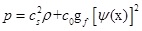
Phase separation between components occurs automatically whenever the interaction potentials are chosen appropriately. The term ψ(x) is a function of the local density. In the single component model, the function of ψ(x) can be varied and different choices could provide various equations of state. Applying the Chapmen-Enskog method which is a successive approximation method, can obtain the macroscopic fluid equation of the LBE model. Meanwhile, the EOS can be stated as below term in Equation 15 [31]:
 |
(15) |
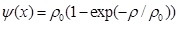
c 0 is a constant term and it is equal to 3.0 for the considered D2Q9 model. In this study, ψ(x) is considered as below in Equation 16:
 |
(16) |
which provides a non-monotonic pressure-density relationship. The body forces can be stated as below in Equation 17:
 |
(17) |
where a is the body force acceleration. The influence of the forces has been incorporated into the LBE model through the momentum variation incorporation in the dynamics of the distribution functions. That means that the velocity ‘u’ in Equation 3 can be replaced with the below in Equation 18 [32]:
 |
(18) |
where Ftotal = F1 + F2. Then, with consideration of averaging of the moment before and after the collision, the whole fluid velocity U can be written as below in Equation 19 [33]:
 |
(19) |
3. NUMERICAL SIMULATIONS
3.1. Problem Statement
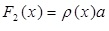
The geometry of the present problem is shown in Fig. (1). It was assumed that fracture domain consists of a two-dimensional enclosure of height H and width W. For the present case, Aspect-Ratio (AR) is defined as the ratio of the width of the enclosure to the height of the enclosure (AR=W/H). The temperatures of the top and the bottom horizontal walls of the domain are maintained at Tc and TH respectively. The two side walls have been considered to be adiabatic i.e., non-conducting. The fracture domain is filled with a Newtonian, incompressible fluid and the flow is laminar.
 |
Fig. (1). Geometry of the present study [2]. |
3.2. Mathematical Formulation
The Boussinesq approximation is used in the natural convection simulation. With this approximation, all material properties of flows are assumed to be constant except the density in the term of gravity. After absorbing the constant part of the gravity into the pressure, the effective external force can be written as Equation 20 [33]:
 |
(20) |
where gy is the acceleration due to gravity, β is the thermal expansion coefficient, T 0 is the reference temperature, which is set as Tc (temperatures of the low temperature wall) in this simulation. ρ 0 is the density of the fluid at T0. Therefore, the macroscopic dimensionless counterpart of the meso-scale governing equations for the natural convection with Boussinesq approximation for incompressible flow is as follows [5, 26]:
Continuity Equation:
 |
(21) |
Momentum conservation:
 |
(22) |
Energy conservation:
 |
(23) |
Equations (21-23) were obtained using the characteristic length H, velocity scale
 time scale t 0 = H/u 0 and pressure scale
 . The dimensionless temperature T* is defined in terms of the wall temperature difference and a reference temperature in Equation 24:
 |
(24) |
Nusselt number, Nu is one of the most important dimensionless parameters in describing the natural convection heat transfer. The local Nusselt numbers at the hot and cold walls are calculated as by Equation 25:
 |
(25) |
Note that the velocity scale in natural convection is proportional to u o. In order to ensure the problem is in the incompressible regime, this value is less than about 0.1. Therefore, appropriate gβ values must be selected [32].
3.3. Boundary Conditions
In practical applications, boundary conditions play important roles in lattice Boltzmann methods in that they will influence the accuracy and stability of the LBE method.
For flow equation, bounce-back boundary conditions were applied on all solid boundaries, which means that incoming boundary populations equal to out-going populations after the collision. For instance, for south boundary by using D2Q9 (Fig. 2) the unknowns are f2, f5 and f6, which are evaluated by using Equation 26 [27]:
 |
(26) |
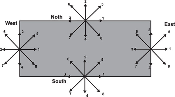 |
Fig. (2). Domain boundaries and direction of streaming velocities for D2Q9 model [34]. |
where n is the lattice local on the boundary. For temperature equation, bounce-back boundary condition (adiabatic) is used on the east and west of the boundaries. For instance, at the east boundary, the following conditions are imposed (Fig. 2) as shown in Equation 27:
 |
(27) |
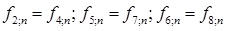
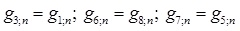
The temperature at the north and west walls are known. Since we used D2Q9, in the south wall (TH), the unknowns are g2, g5, and g6, which are evaluated by using Equation 28:
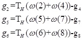 |
(28) |
| Ra |
 H H
|
umax | vmax | |||
|---|---|---|---|---|---|---|
| CFD | LBM | CFD | LBM | CFD | LBM | |
| 103 | 1.0004 | 1.0011 | 3.6464×10⁻⁶ | 2.5534×10⁻⁶ | 3.9684×10⁻⁶ | 4.0012×10⁻⁶ |
| 104 | 2.1581 | 2.1646 | 0.25228 | 0.25531 | 0.26369 | 0.26687 |
| 105 | 3.9103 | 4.0013 | 0.34434 | 0.341231 | 0.37569 | 0.37901 |
| 106 | 6.3092 | 6.3901 | 0.37088 | 0.36977 | 0.40600 | 0.41004 |
3.4. Grid Generation
Grid independence test was carried out for a case of AR = 1 in Re = 105 and Pr =0.71. The results for the surface average Nusselt number (
) at the hot wall in different grid numbers (from 40 to 120 grids) on the lower side of the block surface are plotted in Fig. (3). It is mentioned that the reported number of grids is the number of nodes is defined on each side. As it is observed from the figure, the average Nusselt number values change slightly with the further increase of the nodes from 80 to 120 (less than 1%). The test results (Table 2) reveal the good accuracy of all resolutions greater than 80 nodes per square side. However, to ensure the desired accuracy, the 100-grid case is selected for this study.
| Grids | 40 | 60 | 80 | 100 | 120 |
|
|
3.75 | 3.90 | 3.98 | 4.00 | 4.01 |
| Percent of variation | - | 4% | 2% | 0.50 | 0.25 |
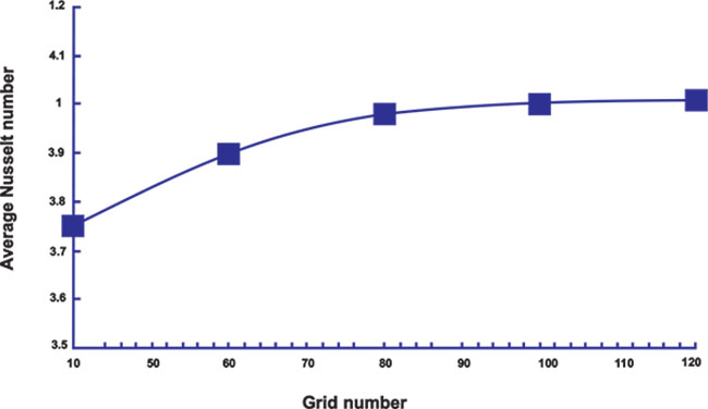 |
Fig. (3).
Evaluation of average Nusselt number (
) on hot wall in different grid numbers.
|
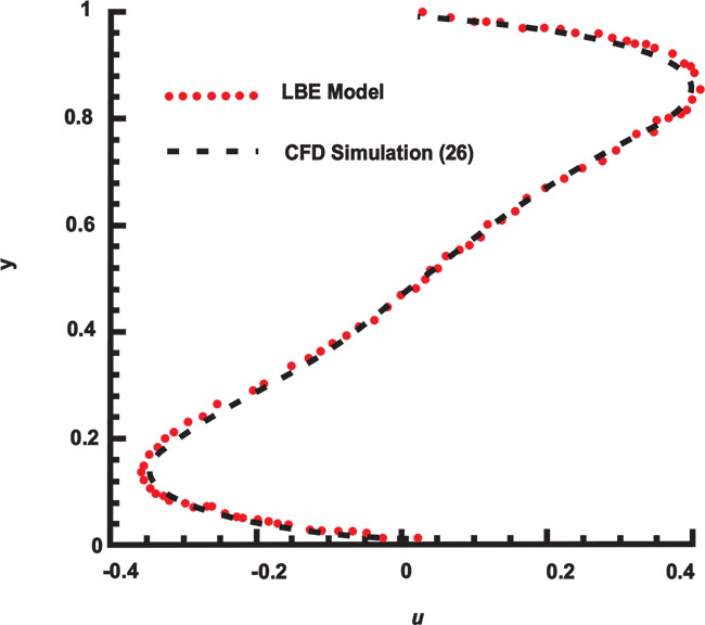 |
Fig. (4). Comparison of variations of dimensionless horizontal velocity between LBE model and CFD results at the middle width of the domain for Pr=0.71 and Ra=105. |
4. RESULTS AND DISCUSSION
4.1. Model Verification
The present numerical code was validated against the results of benchmark CFD [26]. The results are compared in Table 1. As one can see from this table, there are good agreements between two methods. Furthermore, for Pr = 0.71 and Ra = 105, which are reasonable values for petroleum fluid, the dimensionless horizontal velocity (u*) at mid-width (xD= 0.5) and dimensionless vertical velocity (v*) at mid-height (yD= 0.5) of domain are plotted in Figs. (4 and 5) respectively. These figures also show a good agreement between LBE model and CFD results [26]. However, the slight variations in the values are generally due to the employed numerical methods.
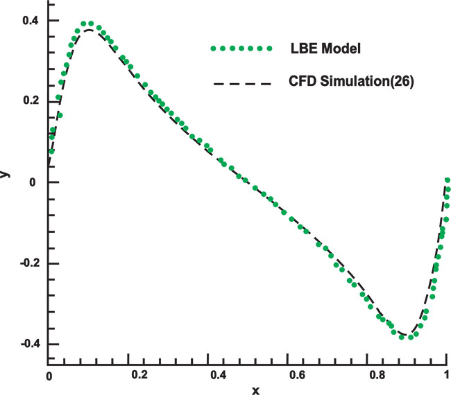 |
Fig. (5). Comparison of variations of dimensionless vertical velocity between LBE model and CFD results at the middle height of domain for Pr=0.71 and Ra=105. |
 |
Fig. (6). Streamline contours for different Ra numbers at Pr=0.71. |
4.2. Single Phase Analysis
Figs. (6 and 7) show streamlines and isothermal contours for Pr = 0.71 at different Ra numbers respectively. As could be seen from Fig. (6) for Ra =104, the flow is symmetrical and has circulating motion in the core region and by increasing Ra, some eddies are then observed at the corners. Fig. (7) also illustrates the isothermal contours, which are symmetrical at the onset of convective motion. However, the contours are indeed more distorted for higher Ra numbers. Moreover, Fig. (8) shows local Nusselt number variations on the hot wall (NuH) at different Ra numbers. As could be easily deduced from this figure, the Nusselt number increases with the increase of Ra number, which indicates the rising heat transfer by natural convection mechanism. Additionally, to gain more quantitative insight into the problem, a summary of average values of local Nusselt numbers and the location with maximum local Nusselt number is presented in Table 3. Values show that both the location of maximum Nusselt number and the average Nusselt of the wall increase with Ra. It should also be mentioned here that average Nusselt numbers are found by surface numerical integration of the local values on the wall.
 |
Fig. (7). Isothermal contours for different Ra numbers at Pr=0.71. |
 |
Fig. (8). Local Nusselt number variations on the hot wall for Pr=0.71 at different Ra numbers. |
| Ra | 104 | 105 | 106 |
| (XD)max | 0.74 | 0.70 | 0.65 |
|
|
1.8 | 3.22 | 5.42 |
Figs. (9 and 10) illustrate streamline and isothermal contours respectively for Pr=0.71 and Ra=105 at different aspect-ratios. In a low AR, temperature field is progressively more linear and thus indicates a proportional increase in the importance of the purely conductive heat transfer mechanism. Because of the no-slip wall boundary condition, a vigorous fluid motion cannot be propagated in the domain in this case. On the other hand, by increasing AR, several convection cells propagated in domain and temperature field became more unsymmetrical.
 |
Fig. (9). Streamline contours at different aspect-ratios (AR) at Pr=0.71 and Ra=105. |
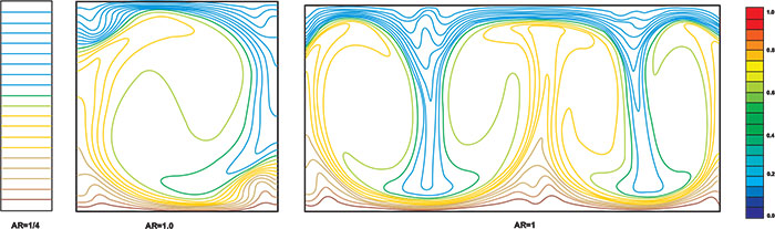 |
Fig. (10). Isothermal contours for different aspect-ratios (AR) at Pr=0.71 and Ra=105. |
4.3. Single Component Multi-Phases (SCMP) Analysis
In petroleum reservoir, one phase may exist in some operation conditions. Because of that, the results of the fluid natural convection with two different phases in a fractured domain are presented in this section which shows heat transfer in the multi-phases model. Other external forces such as drag force, solid/fluid interaction forces, etc have been considered neglected in this simulation.
For the two-phase flow validation analysis, the dynamics of the adherence of two circular droplets have been tested. For instance, initially, two identical droplets with the radius of Ri = 20 were situated very close to each other. The distance of their centers at the centerline of computation domain (xD) is considered 0.5. The higher density section (liquid phase) is inside the droplet and lower density section (vapor phase) is situated outside. The computational resolution is considered 100×100 with gravity free and boundary conditions have been employed periodically in all directions. Once the simulation starts, the droplets coalesce instantly.Fig. (11) represents a snapshot of the droplet shapes at four different lattice times. Moreover, the droplet’s radius at yD = 0.5 as a function of time has been shown in Fig. (12). The droplet’s radius at yD = 0.5 is the distance from the interface node at yD = 0.5 to the center of the domain. The fluctuation of the droplet shape is clear in Fig. (12) and that is due to the surface tension. The relationship of
 has been maintained where Rf represents the final radius of the droplet, and Ri shows the initial radius of two droplets. The result is in a reasonable agreement with other previous investigations [35, 36].
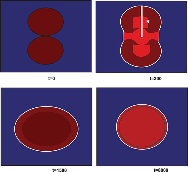 |
Fig. (11). Snapshots of the two droplets cohesion at different lattice times. |
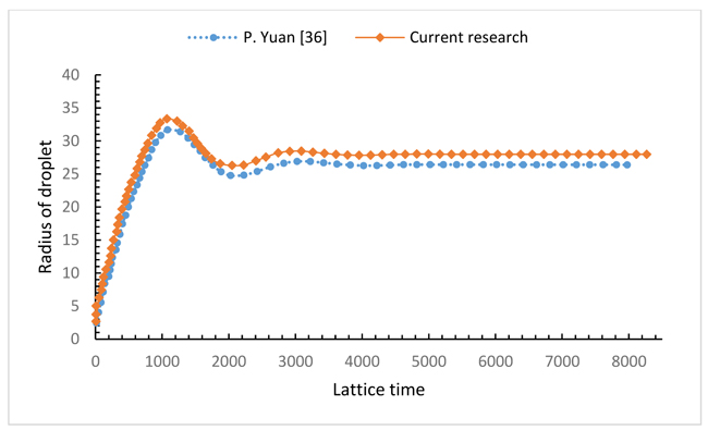 |
Fig. (12). The variation of droplet’s radius as a function of lattice time. |
The existing LBE model can lead to spurious currents which shows the deviation from the reality in the simulation of multiphase flow. These unphysical velocities can be reached to their maximum value at the interface region. The big spurious currents can introduce error in the temperature field and even produce instability in the simulation. The maximum spurious current in this simulation as a function of gf and its comparison with a previously published work [37] is depicted in Fig. (13). Additionally, fluid/fluid interaction strength, gf reduces under some critical value gfC. This shows that a system separates from a single phase to two phases or in other words from heavier liquid phase and a lighter vapor phase. Fig. (14) also represents the density ratio variation versus gf and its comparison with the results in [37]. It is obvious that the LBE method is valid only for the incompressible limit u/cs → 0. This means that u is smaller than 0.13 [31, 33]. In our simulation, to maintain a higher accuracy, maximum velocity needs to be smaller than 0.6 with consideration of the velocity field influence on the field temperature. Therefore, in our simulation, we restrict
 (corresponding to the highest density ratio of 40) which is adequate and valid for many liquid-vapor systems. Obviously, gf cannot be selected a very small value in order to separate phases.
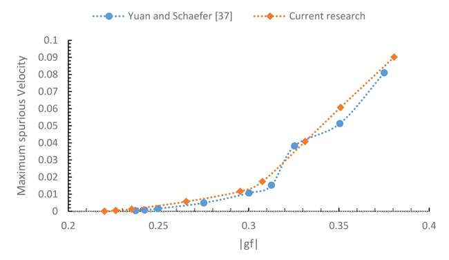 |
Fig. (13). Maximum spurious currents in LBE simulation as a function of gf. |
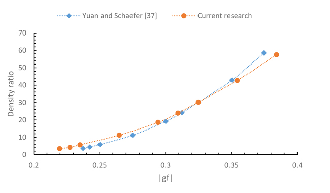 |
Fig. (14). Density ratio in LBE simulation as a function of gf. |
To determine the surface tension numerically, the Laplace law has been introduced in the simulation [38]:
 |
(29) |
where pi and po are the pressure inside and outside the droplet respectively and r is the droplet radius. Therefore, the surface tension of the SCMP model is numerically determined with producing circular droplets with different radii in a gravity free periodic boundary domain and then the slope of the pressure difference versus the inverse of radius relation has been evaluated. Fig. (15) represents the pressure difference versus the inverse of droplet’s radius for , and the concluded linear relation is pretty well satisfied. The surface tension has been calculated with slope and equation 29 calculations. It was found to be 0.0062 in lattice units in the higher correlation coefficient, which was reasonable for petroleum two-phase flow. However, since σ is related to gf, the appropriate surface tension is established with this gf value. Therefore, is applied to the simulation of the thermal multi-phase model.
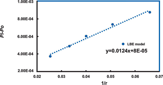 |
Fig. (15). Pressure difference versus the inverse of droplet’s radius for (the correlation coefficient of determination is 0.992). |
To prevent the droplet size expansion or shrinking, we set the initial droplet density of inside/outside close to the maximum/ minimum density value which is obtained from special gf value in Fig. (14). Otherwise, the droplet’s radius is not well-behaved and sometimes the droplet may even expand to the boundaries.
The 100×100 lattices are applied and the boundary conditions set as the previous section. The radius of the droplet which was situated at the center of the domain was 20 lattices. Streamline and isothermal contours at different Rayleigh numbers are brought in Figs. (16) and 17) respectively. As it is obvious in Fig. (16), a central vortex appears as a typical feature of the flow for low Ra values and for the Ra value increment, the vortex tends to become elliptical and streamlines tend to break down. At the same time, as Ra increases the isothermal lines tend to become vertical in the center of the domain and horizontal only in the thin boundary layers near the sidewalls (see Fig. (17). The variation of isotherms indicates the change of the dominant heat transfer mechanism from conduction to convection. This outcome is in agreement with the results of natural convection in a cavity domain which was investigated in previous studies [33].
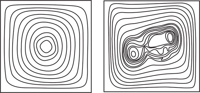 |
Fig. (16). Streamline contours in SCMP LBE model at different Ra numbers. |
 |
Fig. (17). Isothermal contours in SCMP LBE model at different Ra numbers. |
Fig. (18) displays the average bulk Nusselt number variations with the time step at various Rayleigh numbers. The results show that the convection cannot occur in Ra=103 and higher Ra is needed in order to the thermally induced buoyancy can overcome the effects of flow resistance. However, the bulk average Nusselt number rises as the Rayleigh number increases. Moreover, the magnitude of the fluctuations also increases with the Rayleigh number increment. Therefore, the stability of model decreases with increasing the Rayleigh number in the SCMP model.
 |
Fig. (18). The average bulk Nusselt number and the magnitude of its fluctuations versus time step. |
CONCLUSION
In this study, the flow and heat transfer characteristics in a fracture of carbonate petroleum reservoir domain for different Rayleigh numbers with different ranges of aspect-ratio were studied numerically with LBE method. The results of LBE model were compared with the predictions of CFD method and the comparison showed a good agreement with each other. Moreover, the results showed that the average and local Nusselt numbers increase at high Rayleigh numbers. The aspect-ratio affected significantly streamlines and temperature field distribution within the domain. The results showed the conduction heat transfer was dominant in tall fractures, whereas as the width of fracture increased, more natural convection cell propagated in the domain. Finally, the natural convection in a single component mutli-phase model was compared with single phase model. This comparison indicated that stream line and isotherm were affected by second phases in such system. The results also show in SCMP by increasing Ra, streamlines tend to break down and isothermal lines tend to become vertical in the middle of the domain. Moreover, the bulk average Nusselt number and the magnitude of its fluctuations increase as the Rayleigh number increases in the SCMP model.
NOMENCLATURE
|
= Averaged Nusselt number |
| AR | = Aspect-ratio |
| c | = Lattice speed |
| cs | = nLattice sound speed |
| ei | = Particle velocity in i direction |
| f | = Particle distribution function |
| F | = External force |
| feq | = Equilibrium particle distribution function |
| g | = Internal energy distribution function |
| G | = Fluid/fluid internal function |
| geq | = Equilibrium internal energy distribution function |
| gf | = Intensity of fluid/fluid interaction |
| gy | = Gravity acceleration |
| H | = Height of domain |
| LBE | = Lattice-Boltzmann Equation |
| N | = Lattice size |
| Nui | = Local Nusselt number |
| p | = Pressure |
| Pr | = Prandtl number |
| r | = Radius of droplet |
| Ra | = Rayleigh number |
| Rac | = Critical Rayleigh number |
| T* | = Dimensionless temperature |
| t* | = Dimensionless time |
| T | = Temperature |
| U* | = Dimensionless velocity |
| u | = Macroscopic velocity |
| u0 | =Characteristic velocity |
| W | = Width of domain |
| x | = Lattice position |
GREEK SYMBOLS
| β | = Thermal expansion coefficient |
| δij | = Kronecker delta |
| ΔT | = Temperature difference |
| δt | = Time step |
| δx | = Lattice step |
| ρ | = Local mass density |
| σ | = Surface tension |
| τ | = Single relaxation time |
| τT | = Single relaxation time for temperature |
| υ | = Kinematic viscosity |
| χ | = Thermal diffusivity |
| Ψ | = Function of local density |
| ωi | = Weight factor |
| 0 | = Initial |
| * | = Dimensionless |
| C | = Cold |
| eq | = equilibrium |
| H | = Hot |
CONSENT FOR PUBLICATION
Not applicable.
CONFLICT OF INTEREST
The authors declare no conflict of interest, financial or otherwise.
ACKNOWLEDGMENTS
The authors would like to gratefully thank Iranian South Oilfields Company (NISOC) for their technical help and financial support by grant number of 904.