
RESEARCH ARTICLE
Investigation of the Main Factors During Shale-gas Production Using Grey Relational Analysis
Hongling Zhang, Jing Wang*, Haiyong Zhang
Article Information

Identifiers and Pagination:
Year: 2016Volume: 9
First Page: 207
Last Page: 215
Publisher Id: TOPEJ-9-207
DOI: 10.2174/1874834101609160207
Article History:
Received Date: 1/12/2015Revision Received Date: 8/4/2016
Acceptance Date: 22/05/2016
Electronic publication date: 30/09/2016
Collection year: 2016
open-access license: This is an open access article licensed under the terms of the Creative Commons Attribution-Non-Commercial 4.0 International Public License (CC BY-NC 4.0) (https://creativecommons.org/licenses/by-nc/4.0/legalcode), which permits unrestricted, non-commercial use, distribution and reproduction in any medium, provided the work is properly cited.
Abstract
Shale gas is one of the primary types of unconventional reservoirs to be exploited in search for long-lasting resources. Production from shale gas reservoirs requires horizontal drilling with hydraulic fracturing to achieve the most economic production. However, plenty of parameters (e.g., fracture conductivity, fracture spacing, half-length, matrix permeability, and porosity, etc) have high uncertainty that may cause unexpected high cost. Therefore, to develop an efficient and practical method for quantifying uncertainty and optimizing shale-gas production is highly desirable. This paper focuses on analyzing the main factors during gas production, including petro-physical parameters, hydraulic fracture parameters, and work conditions on shale-gas production performances. Firstly, numerous key parameters of shale-gas production from the fourteen best-known shale gas reservoirs in the United States are selected through the correlation analysis. Secondly, a grey relational grade method is used to quantitatively estimate the potential of developing target shale gas reservoirs as well as the impact ranking of these factors. Analyses on production data of many shale-gas reservoirs indicate that the recovery efficiencies are highly correlated with the major parameters predicted by the new method. Among all main factors, the impact ranking of major factors, from more important to less important, is matrix permeability, fracture conductivity, fracture density of hydraulic fracturing, reservoir pressure, total organic content (TOC), fracture half-length, adsorbed gas, reservoir thickness, reservoir depth, and clay content. This work can provide significant insights into quantifying the evaluation of the development potential of shale gas reservoirs, the influence degree of main factors, and optimization of shale gas production.
1. INTRODUCTION
Shale-gas production has drawn worldwide attention over past several years and has changed the energy equation around the world. Shale gas refers to natural gas that is trapped within fine gained sedimentary rocks called shale or mudstone, which can be rich source rocks for oil and natural gas. Shale gas reservoirs are organic-rich formations, and the natural gas in shale gas reservoirs is stored by two mechanisms, free gas and adsorbed gas, which is different from conventional gas reservoir. The permeability of shale gas reservoirs is extremely low on the order of micro-darcy to nano-darcy [1-5].
In order to increase well productivity, production from shale gas reservoirs requires horizontal drilling with hydraulic fracturing to achieve the most economic production. However, there are many uncertain parameters [6-9]. Shale gas reservoirs exhibit complexity across several factors, which can have significant impact on productivity, depending on the production technologies employed. Therefore, to develop an optimal way for quantifying uncertainties and optimization of shale gas production is highly desirable.
Many works have examined the influencing factors on the productivity of shale gas reservoirs. Many researchers [10-12] studied the influencing factors of production performance focus on the geologic features and petro-physical properties of tight gas reservoirs. Wei et al. concerned the impact of TOC on the potential of shale gas in southern China [13]. Fullmer et al. used a pore geometry characterization approach to investigate the influences of micro-porosity on oil recovery [14]. However, Yu and Sepehrnoori paid attention to the impacts of the exclusive features in shale gas reservoirs, such as non-darcy flow behavior, gas desorption, and geomechanics [7]. However, Joshi simulated various fracture models using a fracture simulator to observe their impacts on the well productivity [15]. Previous works show that many scholars have evaluated the development potential of shale gas reservoirs through various methods, but the selected parameters are not comprehensive, or the weight of parameters is determined by subjective assignment method, leading to the reduction in objectivity and accuracy of parameters.
This work focuses on analyzing the main factors during shale-gas production, including petro-physical parameters, hydraulic fracturing parameters, and work conditions on shale gas production performances. Firstly, the key influencing parameters on shale-gas production, from the fourteen best-known shale gas reservoirs in the United States, are selected through the correlation analysis method. Secondly, grey relational analysis (GRA), which is a new analysis method and proposed in the Grey system theory, is used in this work, and the objective weight of each parameter is determined by the grey correlation degree theory. Then, the multiple-attribute evaluation model is established for quantitatively estimating the development potential of target shale gas reservoirs and the impact ranking of main factors. The objective is to provide significant insights into quantifying the uncertainty, characterization of main factors, and optimization of shale-gas production.
2. KEY PARAMETERS FOR DEVELOPMENT OF SHALE GAS RESERVOIRS
Fourteen North American shale plays are used as units of analysis in this paper. The map of them is shown in Fig. (1), and their stratigraphy and depositional environments are labeled in Table 1.
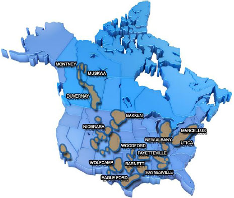 |
Fig. (1). Map of North American shale plays [16]. |
| Shale play | Stratigraphy | Depositional environment |
|---|---|---|
| Bakken | Mississippian | Marine environment |
| Barnett | Mississippian | Marine environment |
| Duvernay | Upper Devonian | Deep-water environment |
| Eagle Ford | Upper Cretaceous | Marine environment |
| New Albany | Late Devonian | Marine environment |
| Niobrara | Upper Cretaceous | Foreland basin environment |
| Utica/Point Pleasant | Upper Ordovician | Basin environment |
| Wolfcamp/Bone Springs | Lower Permian | Marine environment |
| Woodford | Devonian | Shallow marine environment |
| Fayetteville | Mississippian | Shoreface environment |
| Haynesville/Bossier | Middle Cretaceous | Marine environment |
| Marcellus | Later Devonian | Marine environment |
| Montney/Doig | Lower Triassic/Middle Triassic | Marine environment |
| Muskwa | Upper Devonian | Shallow marine environment |
In order to study the impacts of the main factors on gas production, reservoir depth (RD), reservoir thickness (RT), clay content (CLT), reservoir pressure (RP), matrix permeability (MP), porosity (POR), Young’s modulus (YM), total organic carbon (TOC), thermal maturity (TM), adsorbed gas (AG), water saturation (Sw), horizontal well length (HWL), density of hydraulic fractures (Nf), fracture half-length (hf), fracture conductivity (FC), bottom hole pressure (BHP), and the first year decline rate (1st DR) which are easily quantified are selected. These key parameters are obtained from fourteen typical shale gas reservoirs in the United States [17-32], as shown in Table 2.
| Parameters | Unit | Shale Gas Reservoirs | |||||||||||||
|---|---|---|---|---|---|---|---|---|---|---|---|---|---|---|---|
| Bakken | Barnett | Duvernay | Eagle Ford | New Albany | Niobrara | Utica/ Point Pleasant |
Wolf -Bone |
Wood -ford |
Fayett -eville |
Haynesville/ Bossier |
Marcellus | Montney /Doig |
Muskwa | ||
| Depth | ft | 9500 | 6750 | 10500 | 8500 | 3500 | 7500 | 6500 | 8000 | 10000 | 3950 | 10500 | 6250 | 10000 | 8000 |
| Thickness | ft | 49.5 | 300 | 115 | 150 | 125 | 312.5 | 150 | 350 | 170 | 125 | 250 | 175 | 170 | 450 |
| Clay content | wt% | 25 | 35 | 25 | 22.5 | 23.50 | 27.50 | 35.00 | 25.00 | 17.50 | 35 | 40 | 20 | 15 | 20 |
| Reservoir Pressure | psi | 5400 | 3200 | 7950 | 10500 | 850.00 | 5000 | 3250 | 5200 | 3500 | 3500 | 2850 | 7600 | 7510 | 3500 |
| Matrix Permeability | 10-3mD | 3 | 0.225 | 0.29 | 0.128 | 0.008 | 0.5 | 0.0225 | 0.55 | 0.25 | 0.65 | 0.55 | 1.1 | 2.5 | 0.025 |
| Porosity | % | 8.00 | 5.00 | 6.75 | 8.50 | 11.00 | 8.00 | 5.00 | 6.00 | 5.50 | 5.00 | 9.00 | 6.50 | 7.00 | 4.00 |
| Young’S Modulus | 106 psi | 4.00 | 6.00 | 3.80 | 2.88 | 2.50 | 3.20 | 2.30 | 4.80 | 2.51 | 2.45 | 3.50 | 5.50 | 5.07 | 4.50 |
| TOC | % | 10.00 | 5.00 | 6.50 | 4.00 | 13.00 | 5.50 | 2.05 | 5.00 | 6.50 | 7.00 | 2.25 | 6.50 | 5.00 | 5.00 |
| Thermal Maturity | %Ro | 0.75 | 1.45 | 1.80 | 1.38 | 0.96 | 0.98 | 1.65 | 0.90 | 1.30 | 2.50 | 2.15 | 1.60 | 1.83 | 1.90 |
| Adsorbed Gas | % | 25.00 | 35.00 | 10.00 | 15.00 | 15.00 | 35.00 | 20.00 | 40.00 | 25.00 | 50.00 | 15.00 | 50.00 | 20.00 | 10.00 |
| Water Saturation | % | 27.5 | 30 | 20 | 25 | 40.00 | 35.00 | 18.00 | 35.00 | 22.50 | 32.50 | 17.50 | 25.00 | 30.00 | 35.00 |
| Horizontal Length | ft | 5000 | 3250 | 4300 | 4800 | 1800 | 4250 | 6500 | 6050 | 4200 | 3000 | 5800 | 3500 | 6300 | 6800 |
| Fracturing Density | 1/ft | 0.006 | 0.00246 | 0.00512 | 0.00313 | 0.00167 | 0.00259 | 0.00185 | 0.00182 | 0.00262 | 0.00267 | 0.00259 | 0.002 | 0.00254 | 0.002353 |
| Frac Half Length | ft | 450 | 140 | 180 | 230 | 320 | 165 | 280 | 150 | 160 | 420 | 380 | 175 | 260 | 210 |
| Frac Conductivity | md-ft | 160 | 55 | 70 | 140 | 25 | 80 | 130 | 100 | 60 | 250 | 185 | 75 | 180 | 70 |
| BHP | psi | 1000 | 320 | 2000 | 2600 | 350 | 500 | 325 | 520 | 350 | 350 | 350 | 1500 | 500 | 300 |
| 1st Year Decline Rate | % | 65.00 | 50.00 | 55.00 | 70.00 | 60.00 | 80.00 | 70.00 | 60.00 | 65.00 | 60.00 | 50.00 | 64.00 | 54.00 | 71.00 |
Among all the main factors, some parameters may have similarities in data structure, which may result in an increase of workload and the interference of data accuracy. Therefore, in order to make all the main factors be independent, some derivative parameters can be abandoned based on the criterion of correlation coefficient. The correlation coefficient matrix of all the main factors is obtained using the SPSS statistical analysis software, as shown in Table 3. Subsequently, combining with the field experience and setting the liminal value as 0.9, we can see that the selected seventeen parameters have well independence.
| Depth | Thickness | Clay content | Reservoir Pressure | Porosity | Young’S Modulus | TOC | Thermal Maturity | Adsorbed Gas | Water Saturation | Horizontal Length | Frac Density | Frac Half Length | Frac Conductivity | BHP | 1st Year Decline Rate |
|
|---|---|---|---|---|---|---|---|---|---|---|---|---|---|---|---|---|
| Depth | 1.000 | |||||||||||||||
| Thickness | 0.192 | 1.000 | ||||||||||||||
| Clay content | -0.147 | -0.091 | 1.000 | |||||||||||||
| Reservoir Pressure | 0.367 | -0.117 | -0.383 | 1.000 | ||||||||||||
| Porosity | -0.067 | -0.362 | 0.013 | -0.007 | 1.000 | |||||||||||
| Young’S Modulus | 0.099 | 0.618 | -0.107 | 0.170 | -0.344 | 1.000 | ||||||||||
| TOC | -0.518 | -0.360 | -0.289 | -0.327 | 0.428 | -0.219 | 1.000 | |||||||||
| Thermal Maturity | 0.041 | -0.033 | 0.297 | 0.034 | -0.373 | 0.010 | -0.422 | 1.000 | ||||||||
| Adsorbed Gas | -0.541 | 0.088 | 0.201 | -0.057 | -0.321 | 0.219 | 0.021 | 0.024 | 1.000 | |||||||
| Water Saturation | -0.582 | 0.390 | -0.281 | -0.284 | 0.114 | 0.148 | 0.561 | -0.343 | 0.242 | 1.000 | ||||||
| Horizontal Length | 0.570 | 0.505 | -0.021 | 0.154 | -0.384 | 0.093 | -0.745 | 0.172 | -0.401 | -0.312 | 1.000 | |||||
| Fracturing Density | 0.416 | -0.351 | 0.105 | 0.271 | 0.058 | -0.208 | 0.155 | -0.066 | -0.384 | -0.340 | -0.083 | 1.000 | ||||
| Frac Half Length | -0.338 | -0.422 | 0.566 | -0.448 | 0.298 | -0.644 | 0.197 | 0.339 | -0.159 | -0.072 | -0.134 | 0.141 | 1.000 | |||
| Frac Conductivity | -0.071 | -0.158 | 0.555 | 0.030 | -0.139 | -0.408 | -0.458 | 0.681 | 0.138 | -0.258 | 0.220 | -0.052 | 0.619 | 1.000 | ||
| BHP | 0.266 | -0.396 | -0.280 | 0.888 | 0.242 | 0.017 | -0.023 | -0.072 | -0.168 | -0.326 | -0.093 | 0.519 | -0.181 | -0.045 | 1.00 | |
| 1st Year Decline Rate | -0.118 | 0.103 | -0.317 | 0.178 | -0.047 | -0.362 | 0.026 | -0.384 | 0.058 | 0.201 | 0.175 | 0.019 | -0.095 | -0.115 | 0.115 | 1.00 |
3. MODELING OF GREY RELATIONAL GRADE
Assume that the number of shale gas reservoirs to be evaluated is n, denoted as, X={x1,x2,x3,·,xn}, is m, denoted as, V={v1,v2,v3,·,vm}, also known as evaluation indices. Thus, xij (i=1, 2, ·, n; j=1, 2, ·, m) means the j-th parameter of the i-th shale gas reservoir. Then, n shale gas reservoirs and m parameters compose the matrix Z=(xij)n×m, which is the so called evaluation matrix.
To have a uniform standard, the evaluation matrix Z should be normalized in the grey relational analysis [33]. In this paper, the indices are classified into three types: benefit index, cost index, and fuzzy index. The value of the benefit index is the larger the better. The value of the cost index is the smaller the better. The value of the fuzzy index is optimal at the intermediate number.
3.1. Determination of Reference and Comparison Sequences
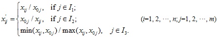
Denote the attribute value of parameter vj to the corresponding ideal target shale gas reservoirs x0 as x0j, then;
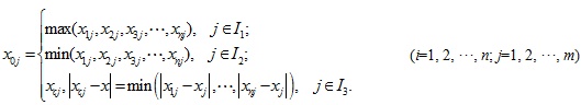
where I1, I2, I3 represent the subscript set of the benefit type, cost type, and fuzzy type, respectively. xj is the theoretical optimal value of parameter vj. The matrix A=(xij)(n+1)×m is the so called evaluation matrix of the set X of target shale gas reservoirs to the set V of parameters.
3.2. Treatment of the Initial Data
In order to cancel out the dimensions, the initial data is non-dimensionalized firstly using the following equation:
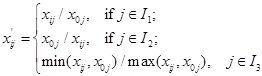
Thus, A'=(xij)(n+1)×m is the initialized matrix of A.
Meanwhile, the range can be calculated using the following equations. The maximal range is
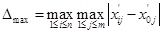
and the minimal range is
3.3. Calculation of the Correlation Coefficients
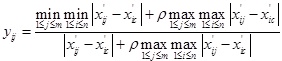
The ideal shale gas reservoir is regarded as the primary sequence, and the shale gas reservoirs to be evaluated are regarded as the subsequence. Then, the correlation coefficient rij can be calculated as follows;
where ρ is the identification coefficient, and it is between 0 and 1. Generally, it is set as 0.5 [34].
3.4. Determining the Weight of Parameters
Choose the parameter which most significantly impacts on the evaluation result as the primary index, and assume the c-th parameter has the most significant influence on the evaluation result. It is denoted as
 . Based on the experiences of shale gas development, the matrix permeability is selected as the primary index in this work. The other parameters are sub-indexes and are denoted as
 , in which j=0, 1, 2, ·, m, but j≠c. The correlative grade between the primary index and the sub-indexes reflects the influence degree of every parameter to the evaluation result, and can be set as the weight of parameter. First, the initial data is also non-dimensionalized firstly using the following equation:
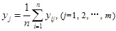
Then, the correlation coefficient of the primary index and the subindex:
Calculate the average value according to the column of matrix Y=(yij)n×m, and then normalization processing is performed:
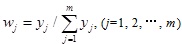
where the matrix W=(w1,w2·,wm)T is the weight of each parameter. The synthetically weighted value, fij = rij×wj, can be regarded as the evaluation value of the exploitation potential of the shale gas reservoirs. A larger weighted value indicates that the shale gas reservoir to be evaluated is closer to the ideal target shale gas reservoir and the development efficiency will be better.
4. RESULTS AND DISCUSSION
According to the Grey Relational Grade model, we select the matrix permeability as the primary index and then the weight of every parameter is obtained as: W = (0.0583, 0.0610, 0.0567, 0.0662, 0.1029, 0.0564, 0.0522, 0.0661, 0.0551, 0.0613, 0.0526, 0.0558, 0.0678, 0.0646, 0.0686, 0.0543, 0.0488)T. The correlative grade of every shale gas reservoir is shown in Table 4. Calculate the synthetically weighted value to achieve F=(fij)n, and then F=(0.6712, 0.5293, 0.5978, 0.5798, 0.6217, 0.5222, 0.5914, 0.5312, 0.5536, 0.6437, 0.6379, 0.5302, 0.6421, 0.6251). We can see that the ranking exploitation potential of each target shale gas reservoir from large to small is Bakken, Fayetteville, Montney/Doig, Haynesville/Bossier, Muskwa, New Albany, Duvernay, Utica/Point Pleasant, Eagle Ford, Woodford, Wolf Bone, Marcellus, Barnett, and Niobrara. This is in accordance with their recovery efficiency 14.0%, 13.5%, 13.0%, 12.5%, 11.0%, 10.0%, 8.5%, 7.0%, 6.8%, 6.6%, 6.0%, 5.6%, 5.3%, and 5.0%, respectively. The calculating results is in accordance with the field result, as shown in Fig. (2), which indicates that the established grey relational grade model is accurate and reliable. Therefore, it can be applied for the evaluation of the exploitation potential of shale gas reservoirs, and the evaluation of the impacting degree of main factors for optimizing the production of shale gas reservoirs.
| Parameters | Shale Gas Reservoirs | |||||||||||||
|---|---|---|---|---|---|---|---|---|---|---|---|---|---|---|
| Bakken | Barnett | Duvernay | Eagle Ford | New Albany | Niobrara | Utica/Point Pleasant | WolfBone | Woodford | Fayett -eville |
Haynesvil le/Bossier |
Marcellus | Montney /Doig |
Muskwa | |
| Depth | 0.4412 | 0.5088 | 0.4279 | 0.4588 | 1.0000 | 0.4832 | 0.5193 | 0.4699 | 0.4341 | 0.8140 | 0.4279 | 0.5312 | 0.4341 | 0.4699 |
| Thickness | 0.3591 | 0.5994 | 0.4011 | 0.4279 | 0.4084 | 0.6201 | 0.4279 | 0.6917 | 0.4449 | 0.4084 | 0.5287 | 0.4493 | 0.4449 | 1.0000 |
| Clay Content | 0.5549 | 0.4660 | 0.5549 | 0.5994 | 0.5796 | 0.5231 | 0.4660 | 0.5549 | 0.7773 | 0.4660 | 0.4438 | 0.6661 | 1.0000 | 0.6661 |
| Reservoir Pressure | 0.5066 | 0.4177 | 0.6725 | 1.0000 | 0.3517 | 0.4877 | 0.4193 | 0.4970 | 0.4279 | 0.4279 | 0.4063 | 0.6436 | 0.6365 | 0.4279 |
| Matrix Permeability | 1.0000 | 0.3503 | 0.3557 | 0.3425 | 0.3333 | 0.3744 | 0.3344 | 0.3791 | 0.3523 | 0.3890 | 0.3791 | 0.4405 | 0.7495 | 0.3346 |
| Porosity | 0.6464 | 0.4776 | 0.5634 | 0.6869 | 1.0000 | 0.6464 | 0.4776 | 0.5231 | 0.4993 | 0.4776 | 0.7328 | 0.5493 | 0.5783 | 0.4393 |
| Young’S Modulus | 0.5399 | 0.4471 | 0.5582 | 0.7123 | 0.8618 | 0.6394 | 1.0000 | 0.4891 | 0.8563 | 0.8907 | 0.5926 | 0.4615 | 0.4772 | 0.5049 |
| TOC | 0.6836 | 0.4476 | 0.4993 | 0.4187 | 1.0000 | 0.4636 | 0.3719 | 0.4476 | 0.4993 | 0.5193 | 0.3762 | 0.4993 | 0.4476 | 0.4476 |
| Thermal Maturity | 0.4160 | 0.5428 | 0.6404 | 0.5256 | 0.4466 | 0.4498 | 0.5946 | 0.4379 | 0.5095 | 1.0000 | 0.7808 | 0.5807 | 0.6487 | 0.6751 |
| Adsorbed Gas | 0.4539 | 0.4111 | 1.0000 | 0.5994 | 0.5994 | 0.4111 | 0.4993 | 0.3994 | 0.4539 | 0.3840 | 0.5994 | 0.3840 | 0.4993 | 1.0000 |
| Water Saturation | 0.5783 | 0.5448 | 0.7996 | 0.6244 | 0.4699 | 0.4993 | 0.9472 | 0.4993 | 0.6917 | 0.5193 | 1.0000 | 0.6244 | 0.5448 | 0.4993 |
| Horizontal Length | 0.6532 | 0.4885 | 0.5756 | 0.6290 | 0.4041 | 0.5708 | 0.9187 | 0.8189 | 0.5660 | 0.4716 | 0.7723 | 0.5068 | 0.8715 | 1.0000 |
| Fracturing Density | 1.0000 | 0.4582 | 0.7720 | 0.5100 | 0.4084 | 0.4672 | 0.4187 | 0.4171 | 0.4695 | 0.4730 | 0.4671 | 0.4279 | 0.4637 | 0.4507 |
| Frac Half Length | 1.0000 | 0.4199 | 0.4539 | 0.5049 | 0.6332 | 0.4405 | 0.5690 | 0.4279 | 0.4362 | 0.8821 | 0.7622 | 0.4493 | 0.5415 | 0.4832 |
| Frac Conductivity | 0.5807 | 0.3900 | 0.4092 | 0.5312 | 0.3565 | 0.4231 | 0.5095 | 0.4539 | 0.3962 | 1.0000 | 0.6573 | 0.4160 | 0.6404 | 0.4092 |
| BHP | 0.4160 | 0.8886 | 0.3697 | 0.3605 | 0.7773 | 0.5549 | 0.8664 | 0.5410 | 0.7773 | 0.7773 | 0.7773 | 0.3840 | 0.5549 | 1.0000 |
| 1st Year Decline Rate | 0.6836 | 1.0000 | 0.8458 | 0.6357 | 0.7495 | 0.5708 | 0.6357 | 0.7495 | 0.6836 | 0.7495 | 1.0000 | 0.6951 | 0.8707 | 0.6277 |
 |
Fig. (2). The relation between integrated weight value and recovery efficiency of the fourteen shale gas reservoirs. |
According to the calculated weight of every parameter, the impact ranking of main factors from more important to less important is the matrix permeability, fracture conductivity, fracture density of hydraulic fracturing, reservoir pressure, TOC, fracture half length, adsorbed gas, reservoir thickness, reservoir depth, clay content, porosity, horizontal length, thermal maturity, BHP, water saturation, and Young’s modulus, as shown in Fig. (3).
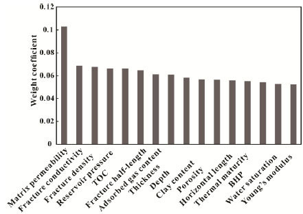 |
Fig. (3). The impact ranking of main factors for the development of shale gas reservoirs. |
CONCLUSION
In this paper, we put forward a new tool to analyze the main factors of shale gas production. Both the definitions and steps are described. The subjective factors and objective factors as well as the interrelation of every parameter are considered synthetically, making the calculation of the weight and evaluation model more reliable. Then, fourteen shale gas reservoirs are used to verify this method and some conclusions are achieved:
- The established grey correction grade model can reasonably, effectively, and objectively reflect the exploitation potential of shale gas reservoirs; it reduces the inaccuracy of shale gas reservoir selection.
- The ranking exploitation potential of the fourteen shale gas reservoirs from large to small is Bakken, Fayetteville, Montney/Doig, Haynesville/Bossier, Muskwa, New Albany, Duvernay, Utica/Point Pleasant, Eagle Ford, Woodford, Wolf Bone, Marcellus, Barnett, and Niobrara.
- According to the parameters of fourteen shale gas reservoirs in the United State, the impact ranking of main factors from more important to less important is the matrix permeability, fracture conductivity, fracture density of hydraulic fracturing, reservoir pressure, TOC, fracture half length, adsorbed gas, reservoir thickness, reservoir depth, clay content, porosity, horizontal length, thermal maturity, BHP, water saturation, and Young’s modulus.
CONFLICT OF INTEREST
The authors confirm that this article content has no conflict of interest.
ACKNOWLEDGEMENTS
This work was supported by the Natural Sciences Foundation of China (Project No. 51474226), the National Basic Research Program of China (2015CB250906) and Important National Science & Technology Specific Projects (2016ZX05047004001).
REFERENCES
| [1] | Akkutlu IY, Fathi E. Multiscale gas transport in shales with local kerogen heterogeneities. Society of Petroleum Engineers Journal 2012; 17(4): 1002-11. |
| [2] | Ghanizadeh A, Aquino S, Clarkson CR, Haeri-Ardakani O, Sanei H. Petrophysical and geomechanical characteristics of Canadian tight oil and liquid-rich gas reservoirs. I. Pore network and permeability characterization Fuel 2015; 153: 664-81. |
| [3] | Liang C, Jiang Z, Zhang C, Guo L, Yang Y, Li J. The shale characteristics and shale gas exploration prospects of the Lower Silurian Longmaxi shale, Sichuan Basin, South China. Journal of Natural Gas Science and Engineering 2014; 21: 636-48. |
| [4] | Yu W, Zhang T, Du S, Sepehrnoori K. Numerical study of the effect of uneven proppant distribution between multiple fractures on shale gas well performance. Fuel 2015; 142: 189-98. |
| [5] | Wang J, Luo H, Liu H, et al. Variations of gas flow regimes and petro-physical properties during gas production considering volume consumed by adsorbed gas and stress dependence effect in shale gas reservoirs. In: SPE Annual Technical Conference and Exhibition; Houston, Texas, USA. 2015.28-30 September; |
| [6] | Rahim Z, Al-anazi HA, Kanaan A, et al. Productivity increase through hydraulic fracturing in conventional and tight gas reservoirs - expectation versus reality. In: Paper SPE 153221 Presented at SPE Middle East Unconventional Gas Conference and Exhibition; Abu Dhabi, UAE. 2012.23-25 January; |
| [7] | Yu W, Sepehrnoori K. Sensitivity study and history matching and economic optimization for Marcellus Shale. In: Proceedings of the 2nd Unconventional Resources Technology Conference; 2014. |
| [8] | Xia L, Luo D, Yuan J. Exploring the future of shale gas in China from an economic perspective based on pilot areas in the Sichuan basin--A scenario analysis. Journal of Natural Gas Science and Engineering 2015; 22: 670-8. |
| [9] | Sun J, Schechter D. Optimization-Based Unstructured Meshing Algorithms for Simulation of Hydraulically and Naturally Fractured Reservoirs with Variable Distribution of Fracture Aperture, Spacing, Length, and Strike. Society of Petroleum Engineers Reservoir Evaluation & Engineering 2015; 18: 463-80. |
| [10] | Khan WA, Rehman SA, Akram AH, Ahmad A. Factors affecting production behavior in tight gas reservoirs. In: SPE/DGS Saudi Arabia Section Technical Symposium and Exhibition; Al-Khobar, Saudi Arabia. 2011.15-18 May; |
| [11] | Mallick M, Achalpurkar MP. Factors controlling shale gas production: geological perspective. In: Abu Dhabi International Petroleum Exhibition and Conference; Abu Dhabi, UAE. 2014.10-13 November; |
| [12] | Pathak M, Deo M, Craig J, Levey R. Geologic controls on production of shale play resources: case of the Eagle Ford, Bakken and Niobrara. In: Paper SPE 1922781 Presented at the SPE/AAPG/SEG Unconventional Resources Technology Conference; Denver, Colorado, USA. 2014.25-27 August; |
| [13] | Wei C, Wang H, Sun S, Xiao Y, Zhu Y, Qin G. Potential investigation of shale gas reservoirs, Southern China. In: SPE Canadian Unconventional Resources Conference; Calgary, Alberta, Canada. 2012.30 October-1 November; |
| [14] | Fullmer S, Guidry S, Gournay J, et al. Microporosity: characterization, distribution, and influence on oil recovery. In: Paper SPE 171940 Presented at the Abu Dhabi International Petroleum Exhibition and Conference; Abu Dhabi, UAE. 2014.10-13 November; |
| [15] | Joshi SR. Simulations of impact of fracture models on shale gas well productivity. In: SPE Annual Technical Conference and Exhibition, 27-29 October; Amsterdam, The Netherlands. 2014. |
| [16] | NUTECH. Unconventional Catalog 2014. |
| [17] | Bustin R, Bustin A, Ross D. Shale gas opportunities and challenges. Search and Discovery 2009; 4038. |
| [18] | Comer JB. Reservoir Characteristics and Production Potential of the Woodford Shale. World Oil 2008. |
| [19] | Chris B, Carpenter J. "Preliminary analytical results: Haynesville Shale in Northern Panola County, Texas. AAPG Datapages". American Association of Petroleum Geologists, 2009. |
| [20] | Chaudhary AS. Shale Oil Production Performance from a Stimulated Reservoir Volume. 2011. |
| [21] | Chalmers GR, Bustin RM, Bustin AA. Geological Controls on Matrix Permeability of the Doig-Montney Hybrid Shale-Gas-Tight-Gas Reservoir. Northeastern British Columbia. Rep 2011. |
| [22] | Hexion. Hexion, "What’s working in the Fayetteville and Barnett Plays? Fracline (2009): Hexion Specialty Chemicals." |
| [23] | Hovey R. The Niobrara Shale. 2011. Hartenergyconferences.com |
| [24] | Hall CD, Debra J, Randy M. Comparison of the Reservoir Properties of the Muska (Horn River Formation) with other North American Gas Shales Rep. Canadian Society of Petroleum Geologists 2011. |
| [25] | Jarvie D. Worldwide Shale Resources Plays and Potential. Worldwide Geochemistry 2010. |
| [26] | Parker M, Dan B, Erik P, Doug G. Haynesvill Shale-petrophysical evaluation. In: Paper SPE 122937 Presented at the SPE Rocky Mountain Petroleum Technology Conference; Denver, Colorado. 2009.14-16 April; |
| [27] | Ross CE. Shale Gas Basics. Crain’s Petrophysical Handbooks 2000. |
| [28] | Scott S. Fayrtteville Shale Overview. Rep. Chesapeake Energy 2008. |
| [29] | Schmidt G, Dunn L, Brown M. The Duvernay Formation (Devenoian): An emerging shale liquids play in Alberta Canada Tech Rep 2012. |
| [30] | Smrecak TA. Introduction to the Marcellus Shale. Paleontological Research Insititution 2011. |
| [31] | Thompson JW, Fan L, Grant D, Martin RB, Kanneganti KT, Lindsay GJ. An overview of horizontal well completions in the Haynesville Shale. In: Canadian Unconventional Resources and International Petroleum Conference; Calgary, Alberta, Canada. 2010.19-21 October; |
| [32] | Warlick D. Assessing the Niobrara Shale Presentation Water Management for Shale Plays Denver, 25, July. |
| [33] | Chan JW, Tong TK. Multi-criteria material selections and end-of-life product strategy: Grey relational analysis approach. Materials and Design 2007; 28(5): 1539-46. |
| [34] | Chen Y, Lu S, Wu Z, Wang W. Application of AHP-GRAP model in the region influence judgment. Journal of Chongqing University 2007; 30(12): 141-6. [Natural Science Edition]. |