
RESEARCH ARTICLE
Induced Microseismicity: Short Overview, State of the Art and Feedback on Source Rock Production
Jean-Pierre Deflandre*
Article Information

Identifiers and Pagination:
Year: 2016Volume: 9
Issue: Suppl-1, M4
First Page: 55
Last Page: 71
Publisher Id: TOPEJ-9-55
DOI: 10.2174/1874834101609010055
Article History:
Received Date: 30/4/2015Revision Received Date: 23/7/2015
Acceptance Date: 12/8/2015
Electronic publication date: 30/06/2016
Collection year: 2016
open-access license: This is an open access article licensed under the terms of the Creative Commons Attribution-Non-Commercial 4.0 International Public License (CC BY-NC 4.0) (https://creativecommons.org/licenses/by-nc/4.0/legalcode), which permits unrestricted, non-commercial use, distribution and reproduction in any medium, provided the work is properly cited.
Abstract
This paper aims at presenting what induced microseismicity is and how it is useful to produce source rock and tight formations. We use our 30-year experience in the field to discuss on data acquisition, processing and interpretation issues. In particular, we establish the difference between hydraulic fracture mapping and long-term monitoring of reservoir mechanical behavior. We comment on advantages and drawbacks of the different monitoring scenarios -from surface acquisition to the use of downhole sensors- while discussing location issues. We illustrate the interest of working on the raw data in order to benefit from valuable information contained into the signal signature. We also refer to examples from the literature to discuss induced seismicity associated with shale play production showing solicitation of conjugate fracture networks or re-activation of faults. Using the north American experience, we introduce the recent debate on anthropogenic seismicity referring to what is currently observed in Oklahoma (US) and western Canada.
INTRODUCTION
This paper illustrates the benefit of monitoring induced microseismicity in different contexts while considering acquisition issues and interpretation challenges. Even if, nowadays, the technique can be considered as mature and the origin of the phenomena as quite well understood, an important challenge remains in its deployment and use while taking into account the knowledge, or the lack of knowledge, we have of the subsurface at the scale we are working: geological heterogeneities, wave propagation velocities, wave attenuation and dispersion effects, uncertainties, etc.
The paper starts with a short review of the pioneering works in different domains (such as hot dry rock geothermal applications or giant gas fields depletion), before focusing on its common use for oil and gas production, especially for shale oil and gas production in the last decade.
To illustrate and understand the origin of induced microseismicity, two different application cases are presented; they correspond to two different monitoring scenarios:
- the short-term monitoring case associated with the hydraulic fracturing of a well and,
- the long-term monitoring case associated with the permanent geomechanical survey of an underground gas storage facility.
Over the last 30 years, IFP Énergies nouvelles (IFPEN) has investigated these different topics; from the general understanding of the phenomena, including research at laboratory scale [1] up to the development of smart downhole equipment for short-time or permanent monitoring [2-5]. These developments were completed by an integrated interpretation approach, including advanced processing of microseismic data [6-8] and allowing to face the challenge of exploiting more or less automatically a significant amount of data (tens of thousands of microseismic files) recorded on a long period of time (several years for instance). The approach has been implemented in the µSICSTM1 software [9]. The aim was to capitalize on the initial training/learning period of a long-term survey in order to improve real-time data interpretation. In this approach, one of the main challenges was to develop automatic processing and interpretation while preserving reliability and quality of treatments and analyses. From case to case, the approach appeared to be efficient enough to spare a lot of engineering time but nevertheless expert analysis remained mandatory to investigate on new types of events. One objective was to deliver some quality control tools for end-users of induced microseismic data; but in this aspect we failed as only a few people (“specialists”) were ready to deal with raw microseismic data.
This paper first discusses data acquisition and processing issues on the basis of the IFPEN’s experience. Then locating issues are addressed also benefiting from the literature.
At that stage, a microseismic event is often reduced to a point in the space characterized by its time of occurrence and the magnitude of its moment. Indeed, clouds of microseisms are too often just used to map faults, fractures, etc. and only in a qualitative way. A lot of relevant information is lost such as frequency content, wave content, signal to noise ratio, signal duration, etc. With some examples we highlight the information that is beyond dots on a map. This information is commonly used by service companies or “experts” to sort the events but generally it is the distribution of events in space and their distribution (number of events) per moment magnitude that are exploited. The space distribution delivers the fracture azimuth and tilt (or its general trends) and the distribution of the number of events per moment magnitude is used to state on the origin/nature of the induced seismicity by interpreting the b-value. Interpretation in terms of induced microseismicity due to hydraulic fracturing or trigged seismicity due to stress redistribution on a fault, may be far from being straightforward.
Then, we go further by illustrating the information that can be exploited in the wave content of microseismic data.
Note that the literature covering microseismic applications and field cases is huge, especially over the last two decades, and only a few references are reported here. A lot of relevant contributors are missing although the reader is strongly recommended to review the literature for each of the subtopics.
Pioneering Works
Microseismicity is nowadays the most efficient technique to state on the dynamic behavior of fractures and faults when considering low magnitude geomechanical phenomena. It corresponds to the energy release under body waves associated with stress release on a surface (geological discontinuity such as a natural fracture or fault plane) or associated with the fracturing and the propagation of the fracture into a continuous medium. By definition microseismicity is similar to natural seismicity but in our context it mainly addresses induced phenomena of low magnitude (less than zero on the Gutenberg-Richter’s magnitude scale): mining, salt leaching, oil and gas field exploitation, fluid underground sequestration or storage and also geothermal applications. Moment magnitudes of microseisms generally range from -3 to 2 on this logarithmic scale: they correspond to extremely low energy levels that are not felt by humans. Just above an event of magnitude 3 is equivalent to a truck vibration, more or less the limit of human perception. Very low energy seismic signals (Fig. 1), from magnitude -3 on the Gutenberg-Richter’s scale can be acquired using appropriate sensors located in the vicinity of the emitting source point (i.e. the hypocenter).
The benefit of microseismic data consists in mapping the zone of mechanical rearrangement within the underground by locating the microseismic sources. In the 70s and 80s, a lot of expertise in microseismic events recording and location was developed for safety issues in the mining domain by instrumenting the galleries to anticipate important stress release effects. A lot of literature came at that time from North America, especially Canada but also from South Africa. Hot dry rock geothermal pilots also contributed to developing the technique; the objective being the optimization of well positioning and the mapping of the underground exchanger surface [11-15]. In parallel, after some seismicity was observed during waste fluid disposal and in association with large scale reservoir depletion [15-19], the oil and gas industry started to use the technique in association with the hydraulic fracturing technique aiming at improving productivity of low permeability formations. Another direct application of the technique deals with hydrocarbon fluid underground storage. With regard to mining, where instrumentation deployment is easy, these application domains had to face new challenges to benefit from the microseismic information because of the great depth and the limited access (wells only) to record the low-magnitude induced phenomena. So to be efficient, it became mandatory to put the sensors very close to the emission zone.
1 µSICS is a registred trademak of IFP Energies nouvelles and GDF-SUEZ for “micro Seismic Interpretation Classification Software”
For that, wireline acoustic sondes equipped with a 3C-sensor were first adapted or designed to collect the information downhole more precisely, in an observation well located close to the injector well or even in the injector well itself [20].
 |
Fig. (1). Example of a microseism recorded on a 3C-geophone located at 1 km depth in a cased well: particle displacement velocity is of few µm/s, event duration is approximately 400 ms [adapted from 10]. |
In the last 40 years a lot of R&D field experiments and applications have been performed in these different domains. They contributed to significant improvements in the technology used for data acquisition and processing, as well as in the methodology, benefiting from concomitant developments of horizontal drilling, well completion tools and well instrumentation. These works also targeted the better understanding of the link between fracture initiation and propagation and induced seismicity through laboratory studies, too. They were strongly supported by universities (Camborne School of Mines - UK, Queen’s University at Kingston - Ontario, TU Delft, The Netherlands), US national laboratories (Sandia, Los Alamos, Laurence Berkeley, etc.) research institutes (e.g. the Gas Research Institute, IFP Energies nouvelles formerly Institut Français du Pétrole), based in the UK, Canada, South Africa, The Netherlands, USA and France. A lot of works in the mining field also come from South Africa and China.
A small activity started and over time small companies emerged developing expertise and/or equipments such as Magnitude, Createch Industrie, Engineering Seismology Group (ESG), Camborne School of Mines Associates (CSMA), Pinnacle and Microseismic Inc. Soon after, a small community appeared with the support of major operators interested in testing the technique such as: Exxon-Mobil, Conoco-Philips, Shell, Statoil, TOTAL. But also Middle East operators such as PDO in Oman and Saudi Aramco (a non-exhaustive list). All these operators had actually mechanical issues to deal with while producing their fields: (chalk compaction in North Sea reservoirs, thermal fracturing because of long term water injection, naturally fractured reservoir, huge depletion in Lacq, Gasli, Californian or Dutch fields or were simply being interested in the potential of the technique for hydraulic fracture mapping. Then major service companies (Schlumberger, Halliburton, Baker Hughes (now part of Halliburton), Weatherford) entered the field too, making important developments while integrating most of the smallest companies with sometimes intermediary stages (ABB buying CSMA prior to sell its activity in the domain to Schlumberger for example). So was the past evolution -here briefly reported in a non-exhaustive way- that contributed in delivering useful tools to optimize hydrocarbon resources production from low permeability formations such as tight reservoirs, shale plays and also coal bed methane production.
Nowadays, an important service is proposed in the field of microseismic monitoring. High-performance instrumentations within a fully integrated approach can deliver in real-time the location of the microseismic events, making it possible to adapt the stimulation treatment program in quasi real-time if necessary.
Application of Microseismic Monitoring in the Oil and Gas Domain
In practice, in the oil and gas domain, one can consider two main applications based on microseismic monitoring:
- Today, the most common application consists in the mapping of the extension of an hydraulic fracture -or a series of- created by injecting an appropriate fluid under pressure into a formation in order to break it and thus to create some fracture permeability. It could also be used during well stimulation tests (performed to restore well productivity) in order to state on the treatment efficiency. But only a few fracturing treatments are effectively mapped,
- The second application corresponds to the “long-term” monitoring of a reservoir in order to understand its mechanical behavior resulting from pore pressure variations [21]. This covers field production including underground gas storage (natural gas and, more recently, CO2 in the frame of Carbon Capture Utilization and Storage pilot tests). Such a monitoring is performed for some cases as for example in France, Italy or The Netherlands where an important survey of the underground has been set in place to follow the oil & gas production activity (including natural gas storage).
To these two application cases correspond quite different monitoring contexts (Fig. 2).
In the first case, the operator knows approximately the time of occurrence of the microseismicity and its a priori location (i.e., in the vicinity of the well perforations at time of injection) as they know where and when they are injecting. It is then easy to position the acquisition network to survey the fracture(s) development or solicitation.
The second case is quite different as the scale of stress release concerns the whole reservoir and its surroundings on a long-term exploitation period (several years and more at least). The higher the permeability of the reservoir, the more global the pressure variation effect: pressure decreases with oil and gas production and pressure increases with fluid injection during sequestration. In the specific case of underground gas storage into saline aquifers, the reservoir pressure cyclically increases and decreases over a year-period as gas is stored in summer and withdrawn in winter for consumption. The higher the variation of pressure, the stronger the mechanical effect for a particular rock type. In the presence of a fault -close to its mechanical equilibrium-, the reservoir pressure variation will modify the effective stresses in the underground either stabilizing the fault or on the contrary making easier its mechanical triggering. Only the occurrence of the second scenario, i.e. mechanical triggering, can be confirmed on the basis of some observed induced microseismic activity.
Short-term Microseismic Monitoring: Hydraulic Fracture Mapping
The left part of (Fig. 2) presents the mapping of a minifrac operation in a mature conventional reservoir. The minifrac technique was developed in the eighties to quantify the effect of a limited injection of fracturing fluid in order to evaluate injection efficiency as well as the risk of having unconfined fractures during a massive injection. The objective was to prevent the fracture from reaching the reservoir-aquifer zone and producing brine instead of the oil. In the particular case of (Fig. 2), it was decided to use the first version of the SIMFRACTM2 tool developed by IFPEN in order to record both the fracturing pressure and the induced microseismicity downhole: this 3-component acoustic tool being equipped with a pressure and a temperature gauge. The tool was lowered-down through the tubing into the stimulated well, just below the perforations and was oriented using surface calibration shots. As suggested by laboratory studies performed in a parallel research project [1, 20], a series of re-injections into the created fracture was performed to acquire more microseismic events, and thus to increase the reliability of fracture mapping. Each re-injection re-opened the recently-created fracture of which the closure was associated with an important induced seismicity. After the latest and major minifrac injection, the survey dragged on during a couple of hours to record the full pressure decline. The aim was to collect the maximum number of microseismic events, especially the discrete and latest ones which, as we observed, often showed high-quality seismic signatures. From the thousands of events that were recorded only a small percentage was effectively located, the other ones being noisy or superposed to other microseisms. Most of the events were within the first 35 m-distance from the wellbore (red ellipse in Fig. (2) - left). The resulting fracture trend was N32°E and its extension was about 310 m while its height was around 100 m. This information was used by the operator to better evaluate the final fracture development. The series of minifrac tests (four at least) was also very informative from the monitoring point of view, suggesting complementary research and development programs to improve the downhole instrumentation and the automatic processing of events [4-9]. In practice, it is of prime
interest to have smart acquisition equipment considering -both the hardware and software- that can lead to identifying in real time the relevant data.
Focusing on shale oil and gas production, multistage hydraulic fracturing of horizontal wells is of course necessary because of the lack of permeability of source rocks. In this context, microseismic monitoring is useful, especially on a new play to evaluate in situ stress directions and to decide on the drilling trajectory path of the horizontal part of the well. Indeed it must be drilled in the direction of the in situ minimum stress to be perpendicular to fracture opening. In practice, the approach consists in performing a minifrac operation in a vertical well at the depth of the horizon to be produced. It corresponds to the injection under pressure of a limited volume of fracturing fluid to initiate a fracture and to start propagating it while recording and locating the associated induced seismicity to map the fracture geometry (extension and azimuth). For example, the result of the mapping of the minifrac test presented in Fig. (2) suggests to drill the horizontal drain in the N122°E direction as this azimuth corresponds to the minimum stress (σhmin) direction. This would position the horizontal drain orthogonal to the fracture network to be developed by multistage fracturing.
 |
Fig. (2). a) Hydraulic fracture mapping of a minifrac experiment in Alberta – Canada [adapted from 20]. The plot gives the distance to the well of each located microseism. b) Long-term microseismic monitoring of an underground gas storage facility in France [adapted from 21]. For both cases, downhole 3C-sensors are located at origin of graph. |
Long-term Microseismic Monitoring: Reservoir Geomechanical Behavior Survey
The right part of (Fig. 2) corresponds to the microseismic activity recorded during an initial ten-month survey of the initial reservoir fill-up at the Céré-la-Ronde underground natural gas storage (located in France). During the period, thousands of seismic/acoustic events were recorded using a downhole network of three geophones placed in a doublet of monitoring wells located at a 20 m-distance. Among this huge amount of events, only a few corresponded to microseismic events. The events were recorded using two types of 3C-sensors: one logging sonde lowered down into the deepest well at 900 m depth and two permanent dowhnole geophones placed respectively at 660 and 680 m depth in the second well. These two sensors were part of a 15-level array permanently deployed for time lapse Vertical Seismic Profiles (VSP’s) in order to map the gas bubble extension. These wells were respectively devoted to neutron logs repetitive measurements at the reservoir level and to the monitoring of the pressure and the fluid composition in an upper aquifer.
In this survey, microseismic monitoring started a month before first gas injection and was performed more or less continuously over a period of 10 years approximately (permanently during the first six years except during drilling or surface seismic acquisitions and occasionally after). Different kinds of seismic or acoustic events were recorded. Among them, 21 microseismic events (such as the one in Fig. (1) of very small magnitudes were acquired during the initial reservoir fill-up. Actually their magnitudes ranged from -1.7 to -0.5 or from -3.7 to -2 depending on model assumptions. The first range resulting from advanced location of hypocenters, may be more reliable. These microseisms were recorded on all the sensors, this was not at all the case for the other signals that were only recorded on one well (except for two small regional earthquakes on June 14th 1994 and October 3rd 1999). Over time we concluded that these microseismic events were directly related to the initial reservoir pressure increase and not to the amount of gas injected, as they have only been recorded in the early times of gas injection, i.e. when the entering gas had to push the brine in place. They were located at the reservoir level or around (violet dots in Fig. (2) right), or far above the reservoir at the level of the upper control aquifer or above it (red dots in Fig. (2) right), i.e., few hundreds of meters above the storage reservoir for the second group. Indeed, microseisms aligned along two main azimuths that correspond to the major faults directions in this area, N157°E and N16°E respectively [21]. They corresponded to effective stress redistribution in the underground, probably stress release on subseismic faults even if such faults were not visible on the seismic acquisitions. It is important to highlight that here no injected fluids or any other one have displaced outside the reservoir to the “seismic active zones”. Contrary to the minifrac example, we can call it “dry” induced seismicity when addressing sparse events not located into the reservoir.
Fig. (3) presents the storage evolution over time in a “stored-volume” versus “reservoir-pressure” graphic representation. The lower part of the graph corresponds to the initial reservoir fill-up (a small amount of gas is stored but the pressure is maximum). The upper part corresponds to the exploitation period when important amounts of gas are injected or withdrawn depending on seasons (generally summer and winter respectively). It can be observed that the microseisms (yellow dots only) disappeared prior to the first withdrawal of gas and did not reoccur as pressure did not reach any higher level during the monitoring period. The last three microseisms were recorded during reservoir pressure stabilization prior to withdrawal. This suggests that a new mechanical equilibrium was reached within the underground. This is not related to the amount of gas injected but to the maxima of pressure successively reached prior compressibility of cushion gas playing its damping role. This period extended over six months. We did not record such events during the two following years but in the same time the reservoir pressure did not reach a new maximum.
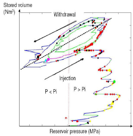 |
Fig. (3). Microseismic events (yellow dots) associated with reservoir pressure increase during initial reservoir fill of an underground gas storage facility in France [adapted from 21]. Other dots correspond to different acoustic phenomena or wellbore signals at reservoir level. |
In the two application cases illustrated here (hydraulic fracturing and the long-term survey of a natural gas storage reservoir), the pressure is the driving force of the system, its induced mechanical effects depend on intrinsic rock petrophysical and mechanical properties and on the in situ state of stress. Dealing with fracturing, the matrix permeability and rock brittleness are key parameters such as fracture propagation criteria. For long-term mechanical effects associated with pore pressure reservoir evolution, key elements are poro-elasticity -including Biot’s theory to state on rock compressibility effects-, and, of course, effective stress redistribution. Increase of reservoir pressure reduces effective stresses, making it possible to damage or break a material or to modify the mechanical equilibrium of a fault (or a fracture), thus triggering it until it reaches a new equilibrium.
Key Issues for Microseismic Data Acquisition
As mentioned above, the technique consists in individually locating each discrete microseism and interpreting the spatial distribution of all as the fracture extension. The challenge is to achieve the location in real time or pseudo real time (i.e., with a short and acceptable on-site delay regarding the operating timing). The quality of this mapping directly depends on the quality of the location of each individual event which depends on:
- Sensor type, their sensitivity and frequency response, their number and location and at least the spatial distribution of the whole acquisition network;
- The acquisition parameters such as the sampling rate and the frequency band-pass of the unit, but also the immunity to ambient noise of the acquisition system that may also have a reliable and unique internal clock for all the seismic channels to be synchronized;
- The local recording conditions such as ambient noise, quality of the coupling between sensors and the formation;
- The reliability and resolution in orientating the 3C-sensors.
In the frame of microseismic monitoring, hydrophones, geophones and accelerometers can be used. In practice geophones are most often used as they allow to record both the compressional and shear waves with a good sensitivity. Hydrophones, limited to compressional waves, are of less interest but if available they can be helpful for the interpretation of wave content. Accelerometers present the advantage of a higher frequency response but this is not systematically a real issue. For downhnole equipment the packaging size is a criterion. Micro Electro Mechanical Sensors (MEMS) are very attractive because of their large and flat frequency response and their small size, but after packaging this second advantage is less determinant and the cost of such sensors remains high in comparison with standard geophones.
In practice, it is common to use 10 Hz-geophone for downhole equipment. It is strongly recommended to systematically use 3C-sensors for data interpretation to better benefit from the full wave content.
Fig. (4) illustrates the main scenarios we may have to record the microseismicity associated with a hydraulic fracturing test. Representation of wave propagation patterns aims at illustrating both wave dispersion and wave amplitude attenuation issues, the rock layers playing the role of a low-pass filter for the wave frequency content. Monitoring options are:
- Monitoring in the treated well (the stimulated one),
- Monitoring in an observation well (any existing well temporary or permanently devoted to this task),
- Subsurface monitoring in a shallow well (a cost-limited observation well),
- Surface monitoring (the cheapest option but, at the same time, the worst).
The closer to the source the better, as low magnitude events can be recorded while collecting higher frequency contents and reducing location uncertainties. But often it is a cost-driven scenario that prevails, having first to confirm the potential of using microseismicity prior to invest a lot of money in equipment. Such a choice is mainly qualitative and may be limiting in terms of location quality; but, in any case, it is useful to prepare further operations at the lowest cost.
Monitoring in the Treated Well
On-tubing permanent downhole geophones Fig. (2) or wireline acoustic tools, such as the SIMFRACTM tool, can be used in the treated well, but they are only operational after pumping. So they are able to map the fracture during closure immediately after injection stops. For the wireline option the sensor has to be removed before any proppant injection. These scenarios are interesting for deep fracturing cases (the most common case) and also when no observation well is available in the vicinity. In the 90s, they were useful for understanding microseismicity phenomena. Nowadays, this scenario is less attractive, especially for the production of source rocks or tight formations where hundreds to thousands of wells are drilled. It may, however, be very interesting in some isolated configuration to have a reference sensor in the treated well in combination with a shallow sensor network, the two networks working in a master-slave configuration. In addition, when possible, this option remains by far the most reliable in terms of location, uncertainties being minimum for different reasons (high frequency content, small distances, good knowledge of velocity models), and in terms of mapping of very low magnitude microseisms.
 |
Fig. (4). Schematic comparison of monitoring network scenarios for a minifrac. The picture corresponds to a 3C-on-tubing geophone to be placed in an exploitation well above the reservoir level for permanent monitoring of an underground gas storage facility (Source: IFPEN-Deflandre and adapted from [4]). |
The use of permanent sensors is better adapted to long-term monitoring allowing to perform time lapse seismic acquisitions (such as Vertical Seismic Profiles) in optimal conditions, as they were initially designed for [3]. The technology has been improved overtime with the development of downhole digital telemetries that strongly reduce ambient-noise effect by comparison with analogical options. This is really valuable in some very noisy locations, such as in an industrial environment that may be the principal limitation to the acquisition of data.
Limitations remain the cost and the number of sensors that can be integrated to the completion. In addition, downhole conditions require a very good casing cementation able to ensure a correct coupling to the formation of each sensor. In addition, sensor positioning has to be optimized according also to the contrasts of acoustic impedance between formation layers.
Over the last decade, the technique benefited from the development of optical sensors that allowed operating at higher temperatures (up to 185 °C), but their use is limited at the moment as well as for many other new but expensive smart-well technologies.
A recent example of such an application is given by the integrated CO2 Capture and Storage pilot run by TOTAL in the Lacq-Rousse area southwest of France. Here, an experimental array composed of a few optical sensors located in the injector well was used in combination with a master network composed of shallow-buried geophone arrays. Objectives were to assess the storage-induced seismicity, survey the seal integrity of the reservoir while distinguishing the induced seismicity from the natural one resulting from local tectonics [22]. The survey network that has been deployed allows to assess the different objectives corresponding to three different scales phenomena. Particularly, it allows to locate with a 250 m-location uncertainty events of magnitude above -0.6 on the Gutenberg-Richter’s scale, allowing to distinguish natural seismicity from the local one due to the huge reservoir depletion. The experimental downhole array allowed detection of nanoseismic events -as reported by the authors because of their extremely low energy level- located around injection in the stimulated reservoir volume and potentially associated with small-scale mechanical disturbances induced by the injection of CO2 in the depleted reservoir.
Monitoring in an Observation Well (a Near-by Well: Close to the Zone of Microseismic Activity)
This option is often the most feasible one, monitoring is operational during and after injection and there is no time limitation as the well is generally devoted to this task [23].
In this scenario, it is common to run a long array of sensors in the well as the tubing may have been removed. Coupling can be optimal by cementing the sensors directly into an open-hole well or into the casing, depending on formations, well completion and safety issues. But, in such cases, sensors are definitively “lost”, they belong to the field owner and this option rules out the use of expensive technologies. The alternative is to work with a service company that will instrument the well for a limited period of time with a more or less smart technology.
Shallow Depth and Surface Monitoring
These options can be used for shallow depth survey, otherwise too much information is lost compared to deep monitoring and location uncertainties strongly increase. When detectable at ground surface or shallow depths, microseisms present a limited frequency content because of wave dispersion and attenuation after propagation on long distances (up to a few kilometers). Between the two, the shallow depth option (500 m for example) is by far the best one as it reduces surface ambient noise effects while taking benefit from being positioned below the low velocity zone -highly dispersive and attenuating for wave propagation. In this case, it can be unrealistic to target high resolution in source location because of the frequency content limitations and consecutive large wavelength values -up to a few hundred of meters in some extreme cases [24].
Microseism Location Issues
Different location techniques can be used depending on the sensor network and the availability of field data (log velocities on one well or a series of wells, 2D, 3D velocity models, etc.). Triangulation techniques rely on the picking of wave arrival times. They are mainly run on the compressional (P) wave arrival times, but they can be applied to the Shear (S) wave arrival times, too. Polarization based techniques require 3C-sensors. They are very efficient techniques to determine the source direction from a 3C-sensor signal and to validate P- and S-wave succession -their respective polarization axis being orthogonal by definition-assuming a similar pathway [7]. Note that, these techniques are operational with only one 3C-sensor and that they deliver the source location with an uncertainty associated to the opposite location in the space centered on the sensor. In such case complementary information is required to determine which of the two solutions is more suitable. For example, the operator knows the sensor is positioned above the stimulated area, then the most probable solution shall be the deepest one. The use of two sensors removes this space uncertainty. This technique has often been used to record deep low magnitude microseisms with a one-level 3C acoustic wireline sonde lowered down into a well. It has allowed the recording of very good quality signals, that were not at all recordable at ground surface.
In the case four 3C-sensors are available, both techniques can be used allowing comparison of source determination. With the triangulation technique the source location is unique for all the sensors. Conversely, the polarization technique results in two solutions per 3C-sensor as indicated above. Here the resolution of sensor orientation is crucial, it requires a high sampling rate and generally best results are obtained by recording a series of surface calibration shots or well perforation shots. If several 3C-sensors are available, the final location can be weighted by the source to sensor distance for each sensor and/or by local velocity-model uncertainties. The quality of the velocity model for both P- and S- waves between sources and receivers is, in addition to the choice of the instrumentation, a key parameter for microseism location. Information about medium properties in terms of wave attenuation and dispersion is also very important for the pre-deployment monitoring feasibility study, but they often remain difficult to obtain. Wavelength of seismic event signal is a parameter to evaluate and consider.
If a 3D-velocity model is available, more sophisticated location techniques based on 3D ray tracing by wavefront construction can be used. Here, the location method relies on the direct computation of polarization and travel time grids (for each sensor), thanks to 3D ray tracing and the minimization of a weighted objective function that leads to the determination of the most probable source [21]. A series of ranked most-probable solutions are obtained, common to all the sensors as for the basic triangulation approach. Experience shows that the most sophisticated approach is not necessarily the best one: a simple but representative wellbore velocity model can be more useful than a complex uncertain 3D one. Calibration shots are determinant in making the decision.
Location reliability depends on the number of sensors that have recorded the microseism, their relative location to the hypocenter and their wave content. A network of four 3C-sensors surrounding the source and “close” to it is better than a dense distant vertical array of sensors, but in practice this is generally more costly to deploy.
Location uncertainties mainly depends on the signal quality and its processing, and of course on the P- and S-velocity models. They can range from 30 m to 400 m depending on P- and S- wave onset quality [24]. They also depend on sensor calibration especially 3C-sensor orientation [25]. This kind of uncertainties is not systematically reported and often under estimated. For example, if the sampling rate for signal digitalization is not high enough, the evaluation of the sensor orientation can be strongly affected independently from any other parameter such as signal to noise ratio, wave amplitudes and so on. Our worst experience is a 40° azimuth change when translating the computation window of only one sample during polarization analysis. In such a case, the remediation option is to re-orientate the different 3C-sensors (permanently installed) using a higher sampling rate acquisition unit. Indeed, the one previously used in our example was appropriate for seismological survey, i.e., very low frequency events (2 ms sampling rate) whereas a 0.2 to 0.5 ms sampling rate acquisition unit should have been used. Of course the difference is in the cost: seismology benefits from a cheap and fit-for-purpose instrumentation whereas microseismicity has not yet cheap solutions. This is a particularly strong limitation for large scale permanent microseismic monitoring where the deployed instrumentation belongs to the operator.
For shale gas or oil production the technique has been quite intensively used in the last years even if a small percentage of hydraulic fractures have effectively been mapped. Multistage fracture treatments can be mapped individually. Mayerhofer et al. [23] show the benefit of using the microseismic technique for field development and especially for well spacing and infill drilling issues. The case corresponds to the multistage fracturing of two horizontal wells in the Marcellus shale. After having fractured well 2H with a series of 7 fracturing stages, a similar fracturing treatment was performed in well H1 while measuring the bottomhole pressure at the wellbore curve level of both wells. In addition to mapping the different fracture sets, microseismic survey suggested communication during injection between the corresponding stimulated rock volumes of both wells and at least between stages 4 to 6 of well H1 with stage 4 of well 2. This communication is understood to be due to a complex fracture network where conjugate fractures may have been solicited as already reported in the Barnett shale [26].
Advanced Microseismic Processing and Interpretation: The Benefit of Wave Content
Beyond the dots (representing the microseisms on a map), a lot of information stands within the wave content itself especially for multicomponent data, making it possible to better characterize and understand the phenomena. First, it allows to describe the focal mechanism when enough information is gathered on the wave radiation pattern. It informs on wave dispersion issues and it can also be used to improve relative location of near-by located events using the doublet or multiplet approach [27, 28]. This can enhance the description of fractures or faults within the reservoir allowing to detect the presence of pre-existing fracture networks or subseismic faults as will be illustrated after. Between two acquisition periods or during a permanent monitoring survey, recently created fractures can also be highlighted by time-lapse signature evolution of microseismic events coming from the “same” location.
Fig. (5) shows high-frequency microseismic events recorded at laboratory scale during the hydraulic fracturing of a rock sample -without any stress applied on the sample (a 40 cm-cubic block). Sensors were positioned at the center of the block faces (mono-axial accelerometers only, as 3C sensors had too low-frequency response at that time to properly record our signals). For the different experiments performed, only a few microseisms were recorded during fracture initiation but most of them occurred later during the propagation stage and mainly during the closure of the fracture. This occurred when pressure dissipates into the rock matrix at the end of injection or when oil escapes the rock sample after the fracture reached the block faces. The upper part of Fig. (5) gives the pressure evolution (up to 11.8 MPa at fracture initiation) and the number of events recorded by time intervals of 2 s (up to 80 events per 2 s at fracture closure when injection stopped). The signals plotted below were recorded: a) during the initiation/early propagation of the fracture; and, b) at fracture closure. During the early propagation of the fracture (a), first-motion polarities appear similar on all sensor recordings. This is not so common, such seismic signatures correspond to a pure tensile mechanism with only a compressional wave recorded on all the block faces. This results from the experimental conditions as no stress was applied on the rock specimen and because of the reasonably good homogeneity of this sandstone rock. In addition, this event occurs at the beginning of the process and was located close to the central injection zone -it is approximately equidistant from the different sensors, time arrivals being quite similar. The signal on the right part of Fig. (5b) was recorded during the propagation of the fracture before injection stopped; it shows different first-motion polarities for the different sensors and a second wave arrival corresponding to a shear wave. In addition, time differences in arrival times clearly indicate that the source is not located any more at the center of the block. Such seismic signatures are more common; they are evidence of a shearing effect on the “fracture plane”. At that time, the fracture was still confined within the block specimen, block failure in two pieces was obtained later -after reinjection at a higher rate into the block sample was performed [1]. Generally, we observe failure in mode II (with a shearing effect) at field scale because of the in situ stress anisotropy.
Fig. (6) is a nice illustration of shear-wave splitting in a medium [29, 30]. The microseism Fig. (6b) has been recorded on an array of 3C-geophones buried in an observation well and processed with the µSICSTM software. It is associated with fluid injection into a fractured reservoir. Once both P- and S- wave arrival times were detected using automatic picking algorithms [8, 9], polarization analysis [7] was applied on the raw data. Eigenvectors are first computed in a reference window automatically associated with the compressional-wave arrival, the aim is to determine the direction of the source (collinear by definition to the polarization axis of the P wave). Then for this particular signal, a focus is put on a second window positioned on the first shear-wave arrival to characterize its polarization (vector RS being its main Eigenvector). In Fig. (6b) the signal is plotted in this specific polarization trihedron. By definition, the vector RS is orthogonal to the P-wave polarization axis previously computed: the P-wave should be in the orthogonal plane defined by the two other eigenvectors (Np and B). In this particular case, the P-wave signal is mainly distributed on the third vector (vector B) only. We also observe a lot of energy on the second vector (vector Np) but arriving with a short delay after the S1 arrival. This second arrival and the absence of energy on the B vector at that time confirm the occurrence of a second shear wave S2. The presence of these 3 orthogonally polarized waves propagating at 3 different velocities is typically representative of the propagation of a microseismic signal through a fractured medium with the main shear wave splitting under two shear waves as schematically illustrated in Fig. (6a). The polarization axis of the first shear wave noted S1 corresponds to the fracture network orientation corresponding to the maximum horizontal stress direction at the time of creation of these fractures. Assuming they were created recently, this direction corresponds to the present maximum horizontal stress direction. If the sensor orientation is reliable, this information can be used for positioning a horizontal well: it has to be drilled perpendicularly to this direction to intersect the fractures.
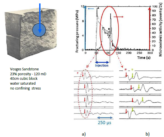 |
Fig. (5). Hydraulic fracturing of a sandstone block at laboratory scale, Fracturing pressure and microseismicity versus time (upper part). Microseisms below a) during early propagation of the fracture and b) at fracture closure [adapted from 1]. |
Looking again at Fig. (1), one may observe that the P-wave frequency is significantly higher than the S-wave frequency. This is typical from the source mechanism but here we have been fortunate to observe it. Such an observation requires the event to occur close enough to the downhole sensor so as to keep its frequency content preserved (and to avoid any strong effect of wave dispersion). This information is of prime interest when looking at source mechanisms [31-33]. Here, the source size has been estimated to be of 8 to 10 m. Most often we suffer from a low-pass filter effect of the ground and P- and S-waves frequency contents appear similar. Part of the information on the frequency content is then lost which may lead to an overestimation of the size of the source.
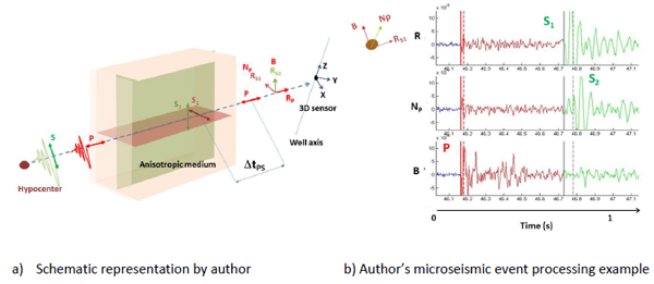 |
Fig. (6). Illustration of shear wave splitting in a fractured formation (vector signification). |
Considering now the identification of the focal mechanism i.e., looking at the ground displacement pattern, it is mandatory, in the author’s opinion, that sensors properly surround the source to be able to state on the mechanism (especially when there is no a priori on the fracture orientation and tilt). Again in practice, we are often limited to one well in the nearby environment of the treated zone (sometimes two wells in the best of cases). If all the sensors are in a unique vertical well (the more common scenario with downhole monitoring) the distance from the source to the array is the key parameter:
- When an important part of the fracture plane is out of the limit of the recording network, part of the fracture cannot be mapped or location uncertainties can be huge (hundreds of meters). In addition, most of the sensors deliver similar information; this brings consistency but in case of a bias it does not reduce the uncertainty.
- When more adapted, we have already observed polarity inversions at mid-length of the sensor array, illustrating differences in the wave radiation pattern associated with the source mechanism. This is valuable information but not enough to properly determine the focal mechanism.
At least, computing seismic attributes at different levels: the seismic channel, the 3C sensor and the event help to automatically define, sort and label different kinds of events such as microseisms, long period events, wellbore events, mono-polarized events, etc. In the object-oriented approach we developed under the µSICSTM software application [6], field exploitation attributes can also be allocated to each event. There is no limit on the origin of those attributes, they can be related to:
- the exploitation data (pressure, low rates, injected or withdrawn volumes, variations of reservoir pressure between wells in a selected period for example, etc.);
- the geology (a petrophysical property of the layer where the microseismic source is located, rock facies, etc.);
- modeling results (reservoir pressure or the effective stress or a delta in the layer where the microseismic source is located at time of occurrence, etc.);
- source parameters; and
- any attribute you can evaluate.
The main difficulty remains in accessing the relevant information to compute the attributes.
On a long-term monitoring survey this approach gives insight on site behavior and is useful to better understand current activity. A basic statistics tool with the possibility of classifying the events using their attributes is integrated into the software. It helps to automatically label new events both on common criteria or site-dependent ones. You can also compare over time the use of different velocity models. We developed and applied this approach on the Céré-la-Ronde natural gas storage monitoring case having a lot of information regarding site exploitation [6-21] and use it on a series or R&D cases. When seismic data are limited to source location and magnitude, the added value is limited even if a lot of operating parameters are available. For instance, it is easy to conclude microseismic events are correlated with pressure levels and at least the horse power delivered for fracking a stage but it remains a very poor and limited analysis!
To conclude on that topic, the integration of seismic attributes (that can be site dependent) into data analysis is of great benefit for data interpretation. Nevertheless, it seems it is not always achieved in some application cases, especially short-term ones, omitting valuable information to better interpretation.
Contribution of Microseismicity to Unconventional Hydrocarbon Production: Focussing on the US Shale Oil and Gas Boom
In addition to the ideal geological context, the shale gas boom in the US seen in the last decade results in part from a series of US specific parameters such as the local context regarding land ownership and regulations (atypical out of the US) but also a very low population density outside main cities and a pioneering and pragmatic enterprising mind. This was enhanced by the geopolitical context and a strong oil & gas industry ready to operate. But it has mainly been possible because of the industrial development of two major technologies in the last 30 years: horizontal drilling and hydraulic fracturing. Within that perimeter, microseismic monitoring is the technique that helps imaging the stimulated rock volume. Then it helps improving safety and efficiency regarding environmental issues, hydrocarbon reserves production and costs associated with “well fracking”, assuming state of the art is strictly applied/respected.
Indeed, the microseismic monitoring technique helps visualizing the results of hydraulic fracturing in terms of fracture dimension and it helps positioning horizontal drains and optimizing field development. It is also the main technique to be used to make possible the evaluation of risk regarding fracture extension and fault reactivation. It is both a control and a design tool. The more it is used, the more we learn on a formation.
The technique has been also put ahead for controlling the risk of fresh-water aquifer contamination from huge (and improbable) fracture extensions (up to 1.5 to 3 km). Probably by analogy to what was proposed formerly when the technique was applied to stimulate conventional reservoir wells. At that time, operators aimed at designing fracture treatments to control fracture extension. They wanted the fracture to remain confined into the pay zone and to not reach the reservoir aquifer located just below the stimulated area. This was not the same problem. At least to mitigate fresh water contamination (shallow depth), it is better, in the author’s opinion, to first focus on well integrity issues or simply on surface contamination problems. Surface contamination should not occur if waste management follows state of the art and regulations. Dealing with well integrity issues, using the microseismic technique in combination with high resolution well seismic at wellbore can be valuable [34].
Nowadays, after more than a decade of intense shale-play exploitation and important feedback on microseismic monitoring, new discussion topics are taking place. The intensive hydraulic fracturing of dense horizontal well pads develops large fractured rock volumes and significantly modifies in situ effective stresses making the re-activation of faults intersecting the stimulated rock volume possible -as illustrated by Snelling et al. [35]. In this case, the b-value interpretation (the slope of the distribution of the number of events per magnitude range) helps making the difference between hydraulic fracture development and fault re-activation with higher magnitude events corresponding to fault re-activation.
Over the last years, anthropogenic seismicity associated with shale plays production has been more and more reported [36], some events are directly associated with the fracturing fluid injection into the source rock as at Blackpool, in the UK [37], but major ones more often result from waste fluid re-injection in another formation. Since 2014, Alberta and British Columbia (Canada) and Oklahoma (US) [38, 39] are “under monitoring” respectively, for a 4.4 magnitude event near Fox Creek, Alberta, in January 2015 and because of a significant increase in the number of earthquakes of magnitude greater than 3 in the whole state (Fig. 7), [40]. Indeed, in Oklahoma up to 585 earthquakes above this threshold have been recorded in 2014 with hypocentre locations ranging from 2 to 10 km depth, the average depth being 6 km [40]. It is reported that this induced seismic activity is linked to the injection of waste drilling or fracturing fluids into disposal wells and not directly associated with hydraulic fracturing operations. It is often suggested that hydraulic fracturing is not supposed to trigger felt earthquakes except in the presence of a major fault that is close to its equilibrium (in other words, a low variation of effective stress may be enough to trigger it). Note, also, that permeable faults depending on injection rate can be aseismic until a certain point. This may depend on the injection rate, the fluid injected and the ability of the formation to accommodate the pressure increase. A lot of R&D studies and measurements are now on-going to mitigate anthropogenic seismicity at that level of magnitude.
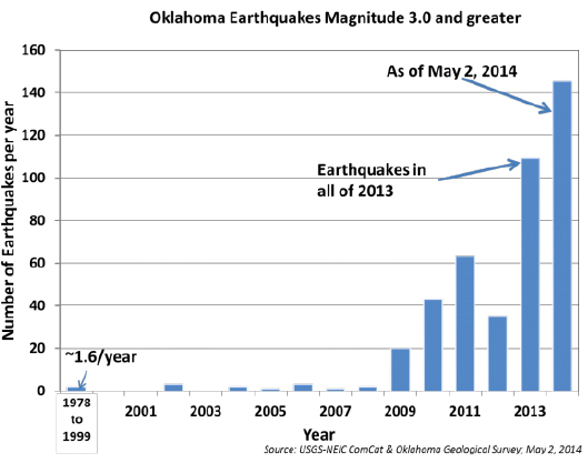 |
Fig. (7). Oklahoma earthquakes magnitude (3.0 and greater) survey [38]. |
Monitoring the induced microseismicity may allow to fix acceptable thresholds for operations especially for waste fluid disposal. Quantitative microseismicity helps to better understand the phenomena and describe the site (higher resolution) especially when natural fracture systems and faults are not visible on the seismic. When only quantitative, it is useful for reporting potential hazard having a quick interpretation of on-going facts. A key issue is the amount of energy (absolute and/or per unit of time) that is dissipated into the ground regarding the ability of the underground to adapt to it. Forecasting is not “a piece of cake” as both the initial state of stress and the formation properties are not known. The same applies for fault re-activation as no one can predict the gap between the equilibrium domain and the point of re-activation. Regarding the energy involved in a massive fracturing treatment, fault-reactivation may generate felt seismic events when the solicited fault plane is important. But real time monitoring and interpretation of low magnitude events may help to mitigate such a scenario by stopping/adapting the treatment. This could be the case if the microseismic activity concentrates in a zone that is not coherent with the fracking process or if there is no induced microseismicity at all. In such a case one can expect a permeable fault to be penetrated by the injection fluid, stopping injection could be the decision to take.
Again, anthropogenic microseismicity/seismicity is not only associated with hydraulic fracturing of source rock plays to produce unconventional hydrocarbon resources. It also concerns mining, salt leaching, conventional reservoir depletion, dam filling, geothermal applications, waste fluid re-injection into the ground, underground fluid storage (natural gas, hydrocarbon liquids, CO2), etc. At least, it may also address underground energy storage if pressure/effective stress variations are not managed in parallel. In 2013, a synthesis of presumed anthropogenic induced earthquakes as reported in the literature was established by Davies et al. [37]. At the time, the survey showed that shale gas fracking and waste disposal remained below mining activities, oil & gas field depletion and reservoir impoundment, both in terms of number of events and maximum of magnitudes. This may change over time when looking at the USGS-OGS survey presented in Fig. (7).
CONCLUSION
Induced microseismicity delivers valuable information on what is on-going underground when effective in situ stresses are affected by pressure changes. The technology is available to record very low magnitude events located deep in the ground, especially using (digital) downhole equipment. Data interpretation is a real issue, it relies firstly on appropriate and reliable acquisition systems and secondly on a good knowledge of wave propagation velocities between microseismic sources and sensors. Depending on the attention paid for acquisition and processing, deliverables are more or less qualitative. The minimum output is the location of hypocentres sized in magnitude with an evaluation of the location uncertainty, the threshold in lower magnitude being directly dependent from the distance between the emitting zone and the sensors. The more sensitive the acquisition network, the better the characterization of the site. To really benefit from the potential of monitoring induced seismicity, it is mandatory to work on the raw data and to exploit signal content/signature in terms of wave and frequency content, signal wavelength, wave polarization properties, etc. which can inform on the fractured structure of a layer, for example. As there are no two sites alike, monitoring induced microseismicity should be part of the first-level monitoring panoply to be deployed when affecting the underground state of stress, regardless of the origin of the perturbation (fluid injection or withdrawal, permanent of temporarily fluid storage, mining, salt leaching, etc.) and whatever the purpose (fossil energy production, energy storage, waste fluid storage including CO2, etc.).
In addition, to better characterize the in situ state of stress and to evaluate optimal horizontal drain azimuth and to optimize field development, the added value is directly associated with the potential hazard of triggering a felt earthquake as it is nowadays reported in some North American states/provinces.
A lot of applied R&D work should be carried out to mitigate felt induced seismicity reported as anthropogenic seismicity especially in identifying more appropriate field patterns that allow a formation to accommodate with massive injection and pressure changes. It will probably harm productivity from case to case but it might also be a factor of greater efficiency especially when considering the number of fractured stages or wells that do not produce a lot. The question is can induced microseismic monitoring help improving well productivity by contributing to develop smarter production scenarios with less wells? Is time lapse re-fracking a relevant strategy for a more sustainable approach? In the field of waste fluid re-injection into disposal wells, operating conditions have to be adapted to local context to avoid felt seismicity to be triggered. A state of the art and guidelines have to be established as it is on-going for a decade now for gas production and also storage in The Netherlands [41]. There the possible occurrence of induced seismicity is ranked on a 3-level scale for risk assessment and risk management with appropriate guidelines to be applied at each level. The objective is to remain below an acceptable threshold of induced seismicity while considering the economic and strategic benefits of the gas exploitation.
CONFLICT OF INTEREST
The authors confirm that this article content has no conflict of interest.
NOTES
1 µSICS is a registred trademak of IFP Energies nouvelles and GDF-SUEZ for “micro Seismic Interpretation Classification Software”
2 SIMFRAC is a trademak of IFP Energies nouvelles
ACKNOWLEDGEMENTS
The author thanks Dr. Florence Delprat-Jannaud for reviewing the text and is indebted to all his previous colleagues and co-authors for their long-term collaboration on different topics during 30 years.
REFERENCES
| [1] | Deflandre JP. Laboratory analysis of acoustic emission associated with the hydraulic fracturing of sandstone samples - The problem of fracture location. Oil Gas Sci Technol 1989; 44(5): 673-91. |
| [2] | Sarda JP, Wittrisch C, Perreau Ph, Deflandre JP. Downhole frac monitoring system developed. Oil Gas J 1987; 4: 44-6. |
| [3] | Deflandre JP, Laurent J, Michon D, Blondin E. Microseismic surveying and repeated VSP's for monitoring an underground gas storage reservoir using permanent geophones. First Break 1995; 13(4) |
| [4] | Deflandre JP, Vidal-Gilbert S, Wittrisch Ch. Improvements in downhole equipment's for fluid injection and hydraulic fracturing monitoring using associated induced microseismicity In: paper SPE 88787, ADIPEC; October 10- 13; Abu Dhabi. 2004. |
| [5] | Thérond J-F, Deflandre JP, Grouffal C. Method intended for detection and automatic classification, according to various selection criteria, of seismic events in an underground formation US Patent no. 6.920.083 B2, 10/262.966, 2005 [July 19,]; European patent no. 02292258, March 10, 2002. |
| [6] | Deflandre JP, Dubesset M. Identification of P/S wave successions for application in microseismicity. Pure Appl Geophys 1992; 139(3/4) |
| [7] | Deflandre JP. Method for analysing acquired signals for automatic location thereon of at least one significant instant US Patent no 6.598.001 B1–, European patent no. 00402033.5-2213, July 22, 2003. |
| [8] | Deflandre JP. Procédé pour localiser l'origine spatiale d'un événement sismique se produisant au sein d'une formation souterraine European patent no 09290357.4 - 1240,, May 13, 2009. |
| [9] | Deflandre JP, Delaplace Ph, Huguet F. Permanent Passive Seismic Monitoring for Reservoir Management: the µSICSTM Approach EAGE/SEG Research Workshop on Reservoir Rocks. Pau, France.. 2001. |
| [10] | Deflandre JP, Huguet F. Microseismic monitoring on gas storage reservoirs: a ten-year experience In: 17th World Petroleum Congress, Block 3 Forum 19; September 1st - 5th; Rio Brazil. 2002. |
| [11] | Pearson C. The relationship between microseismicity and highpore pressures during hydraulic stimulation experiments in low permeability granitic rocks. J Geophys Res 1981; 86(B9): 7855-64. |
| [12] | Albright JN, Pearson CF. Location of hydraulic fractures using microseismic techniques In: paper SPE9509, 55th Annual Fall Technical Conference and Exhibition; September 21-24,; Dallas, Texas. 1980. |
| [13] | Jupe AJ, Green AS, Wallroth T. Induced microseismicity and reservoir growth at the Fjällbacka Hot Dry Rocks project, Sweden Int J Rock Mech Min Sci Geomech Abstr 1992; 29(4): 343-54. |
| [14] | Cornet FH, Jianmin Y. Analysis f induced seismicity for stress field determination and pore pressure mapping. Pure Appl Geophys 1995; 145(3/4) |
| [15] | Phillips WS, Rutledge JT, House L, Fehler MC. Induced Microearthquake patterns in hydrocarbon and geothermal reservoirs: six case studies. Pure Appl Geophys 2002; 159: 345-69. |
| [16] | Segall P, Grasso JR, Mossop A. Poroelastic stressing and induced seismicity near the Lacq gas field, southwestern France. J Geophys Res 1994; 99: 15423-38. |
| [17] | Suckale J. Moderate-to-large seismicity induced by hydrocarbon production. Leading Edge (Tulsa Okla) 2010; 29(3): 310-7. |
| [18] | Grasso JR, Wittlinger G. Ten years of seismic monitoring over a gas field. Bull Seismol Soc Am 1980; 80(2): 450-73. |
| [19] | Maury VM, Grasso JR, Wittlinger G. Monitoring of subsidence and induced seismicity in the Lacq gas field (France): the consequences on gas production and field operation. Eng Geol 1992; 32: 123-35. [Elsevier Science Publishers B.V., Amsterdam.]. |
| [20] | Sarda JP, Perreau P, Deflandre JP. Acoustic emission interpretation for estimating hydraulic fracture extent: laboratory and fields studies In: SPE - 63rd Annual Technical Conference and Exhibition of the Society of Petroleum Engineers Proceedings; October 2-5; Houston. 1988; pp. 113-22. SPE 18192. |
| [21] | Deflandre JP, Dubos-Sallée N, Huguet F. Passive seismic monitoring of gas storage: challenges for improving interpretation and reducing uncertainties In: EAGE Workshop on Passive Seismic. Limassol, Cyprus 2009. |
| [22] | Payre X, Maisons C, MarblA(c) A, Thibeau S. Analysis of the passive seismic monitoring performance at the Rousse CO2 storage demonstration pilot“ Energy Procedia 2014; 63: 4339-57. |
| [23] | Mayerhofer MJ, Stegent NA, Barth JO, Ryan KM. Integrating fracture diagnostics and engineering data in the marcellus shale In: SPE Annual Technical Conference and Exhibition held in Denver. Colorado, USA. 2011.30 October–2 November 2011.; Colorado, USA.: 2011. |
| [24] | Fabriol H, White D, Maxwell S, Deflandre JP, Jousset Ph. Microseismic monitoring of CO2 injection at the Weyburn oil field, Saskatchewan, Canada In: International Conference on Green house Gas Control. 2125-9. |
| [25] | Deflandre JP, Andonov LJ, Fabriol H, White D. Induced microseismicity and CO2 injection at the weyburn oil field: Improvements in source location In: 8th GHGT, International Conference on Green House Gas Control; Trondheïm, Norway. 2006. |
| [26] | Maxwell SC, Waltman C, Warpinski N, Mayerhofer M, Boroumand N. Imaging Seismic Deformation Induced by Hydraulic Fracture Complexity 2006. SPE 102801. |
| [27] | Poupinet G, Ellsworth WL, Fréchet J. Monitoring velocity variations in the crust using earthquake doublets: An application to Calaveras Fault, California. J Geophys Res 1984; 89(B7): 5719-31. |
| [28] | Kendall JM, Bastow I, Raymer DG, Wuestefeld A. Characterization of fractures and faults: a multi-component passive microseismic study from the Ekofisk reservoir. Geophys Prospect 2014; 62(4): 779-96. |
| [29] | Crampin S, Lovell JH. A decade of shear-wave splitting in the Earth’s crust: what does it mean? What use can we make of it? and what should we do next?” Geophys J Int 1991; 107: 387-407. |
| [30] | Crampin S, Peacock S. A review of shear-wave splitting in the compliant crack-critical anisotropic Earth. Wave Motion 2005; 41: 59-77. |
| [31] | Mizuno T, Nakai M. Development of a database of shear-wave splitting of the crustal earthquakes”, OpenSWS, Bull. Bull Earthq Res Inst Univ Tokyo 2005; 80: 43-52. |
| [32] | Brune J N. Tectonic stress and the spectra of seismic shear waves from earthquakes J Geophys Res, v 1970; 75(26): 4997-5009. |
| [33] | Madariaga R. Dynamic of an expanding circular fault. Bull Seismol Soc Am 1976; 66(3): 639-66. |
| [34] | Deflandre JP. Method for seismic monitoring of an underground zone under development allowing better identification of significant events US Patent no. 6.049.508 A-, 2000 [April 11]; European patent no. 98402975.1-2213. |
| [35] | Snelling P, de Groot M, Craig C, Hwang K. Structural controls on stress and microseismic response - A horn river basin case study In: Society of Petroleum Engineers. 2013. In: SPE 167132 URTEC; November 5; Calagary, Alberta, Canada.. 2013. |
| [36] | Shale Gas Extraction in the UK: A Review of Hydraulic Fracturing. June 2012 - DES2597. |
| [37] | What size of earthquakes can be caused by fracking? 2013; “Induced seismicity and hydraulic fracturing for the recovery of Hydrocarbons”, Marine and Petroleum Geology 45; 07/31/15; 2013; pp. 171-85. Available at: http://www.sciencedirect.com/science/ article/pii/S0264817213000846. ISSN 0264-8172. |
| [38] | USG OGS Joint press Realease May 5th 2014 2014 [ 07/31/15.]; Available from: (http://www.okgeosurvey1.gov/ media/press/Full_USGS- OGS_Statment_05022014.pdf) |
| [39] | McNamara D E, Rubinstein J L, Myers E, et al. Efforts to monitor and characterize the recent increasing seismicity in central Oklahoma 2015 [June 2015.];628-39. |
| [40] | Darold AP, Holland AA, Morris JK, Gibson AR. (2015), Oklahoma Earthquake Summary Report 2014, Okla. Geol. Surv. Open FileReport, OF1, 2015. |
| [41] | Muntendam-Bos A G, Roest JP A, De Wall J A. A guideline for assessing seismic risk induced by gas extraction in the Netherlands The Leading Edge 2015; 672-7. |